
Verification - Input Commands
Introduction
This document presents verification tests for the input commands available in the software.
Tests are continuously added to a database which currently contains over 500 tests. The tests consist of small models, often based on a single element or component, and are designed to test a specific feature of the input command under consideration. Each test is associated with at least one target which is defined based on analytical solutions, results from other numerical methods or in a few cases, results at implementation to ensure consistency in results for new solvers. The targets are automatically checked after running the tests in the database with a new solver.
Version control
The tests presented in this document are subjected to version control, meaning that the tests are run and evaluated prior to release of a new solver. This document is updated in conjunction with official releases of the software.
*ACTIVATE_ELEMENTS
Activation and deactivation of elements
"Optional title"
coid, entype, enid, $t_{birth}$, $t_{death}$, $\xi$
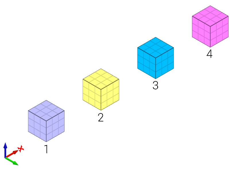
Activation and deactivation of elements in *ACTIVATE_ELEMENTS are verified in this test.
Tested parameters: $t_{birth}$ and $t_{death}$.
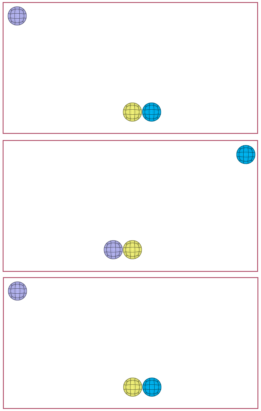
Four CHEX elements are positioned along the X-axis as displayed in Figure 1. The activation and deactivation of each element is presented in Table 1.
| Element ID | 1 | 1 |
|---|---|---|
| 1 | 0 | - |
| 2 | t | - |
| 3 | 0 | t |
| 4 | t | - |
An initial velocity in the X-direction is imposed on element 1. Once element 1 has passed the position of element 2, element 2 and 4 are activated and element 3 deactivated. Element 1 continues to translate along the X-axis and then collides with element 4, bounces back, and eventually collides with element 2.
The positions of the elements at initiation and termination are checked.
Tests
This benchmark is associated with 1 tests.
Rebar elements
"Optional title"
coid, entype, enid, $t_{birth}$, $t_{death}$, $\xi$
Deleting elements created by *COMPONENT_REBAR with *ACTIVATE_ELEMENTS are verified with this test.
One rebar grid is created using *COMPONENT_REBAR. The grid is given an initial velocity in x-direction. A function is set so that when the center of gravity of all rebar elements which are > 0 in X-direction, the rebar elements will be deactivated, see Figure 1.
The mass of the rebars at initiaton and termination is checked.
Tests
This benchmark is associated with 1 tests.
Strength of elements prior to activation
"Optional title"
coid, entype, enid, $t_{birth}$, $t_{death}$, $\xi$
Strength prior to element activation in *ACTIVATE_ELEMENTS is verified in this test.
Tested parameters: $\xi$.
Four CHEX elements are positioned as displayed in Figure 1.
Element 1 and 3 are merged to element 2 and 4 respectively. Element 2 and 4 are given an initial velocity in the X-direction and element 1 and 3 are not activated until half the simulation time has passed. Before activation, element 1 has full strength while element 3 has no strength. Once the elements are activated, there should be no gap between element 1 and 2.
The positions of the elements at initiation and termination are checked.
Tests
This benchmark is associated with 1 tests.
*ADD_MASS
Rotating discs
"Optional title"
coid, entype, enid, $m_{add}$, distribution
The different mass distribution options available in *ADD_MASS are verified in this test.
Tested parameters: madd and distribution.
Three discs are spinning around their central axes. In the first disc, the added mass is distributed over the nodes (option 0). In the second and third disc, the added mass is distributed over the area (option 1 and 2). An added mass equal to the actual mass of the disc is used.
The kinetic energy due to the added mass for each disc is calculated as:
$$ E_k = \frac{1}{2} \cdot I \cdot \omega^2 $$
$\omega$ is the angular velocity and $I$ is the moment of inertia, defined as:
$$ I = \frac{1}{2} \cdot m \cdot r^2 $$
$m$ is the mass and $r$ is the radius of the disc.
The kinetic energy of each disc at termination is checked.
Tests
This benchmark is associated with 1 tests.
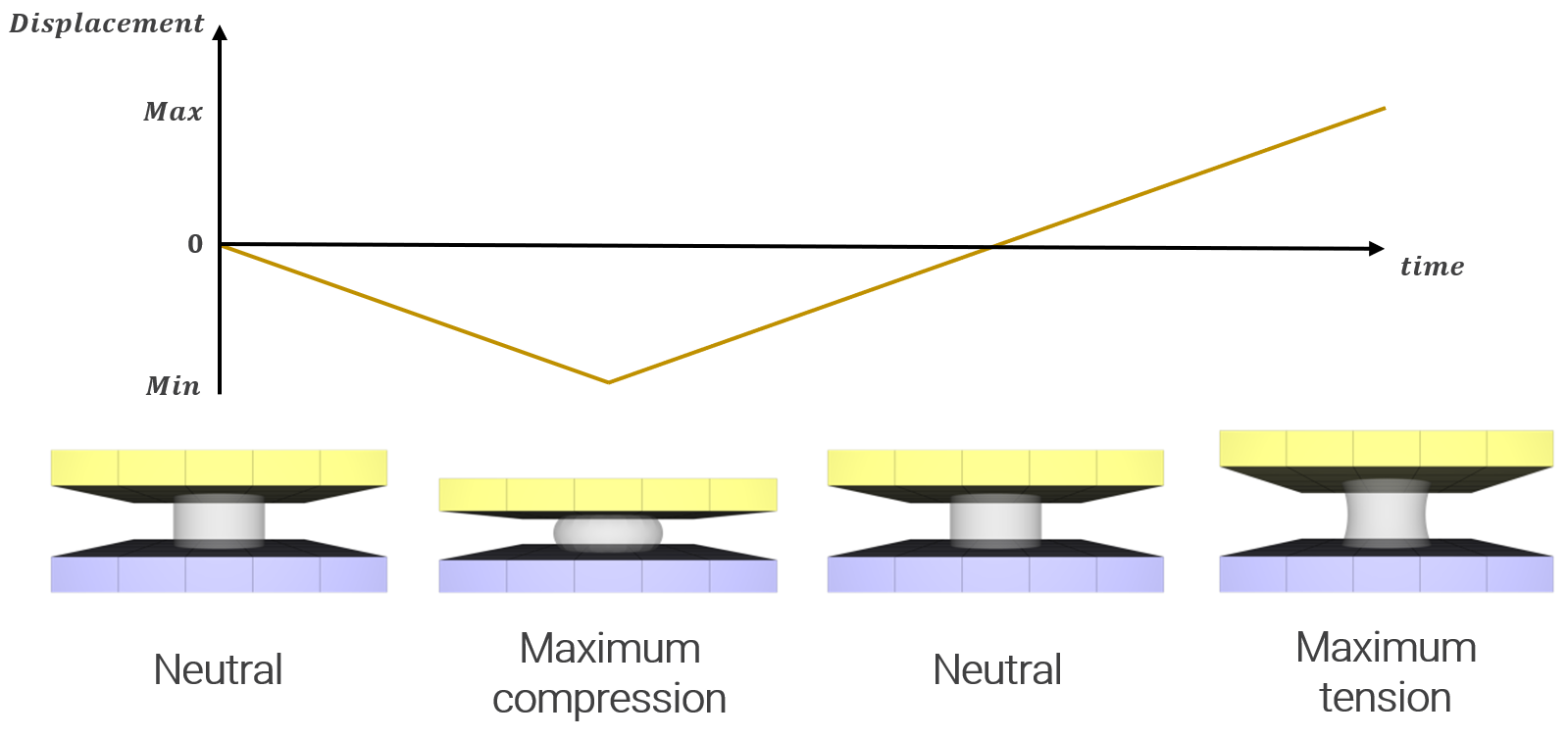
*BC_MOTION
Activation and deactivation
"Optional title"
coid
entype, enid, bc${}_{tr}$, bc${}_{rot}$, csysid${}_{tr}$, csysid${}_{rot}$, $t_{beg}$, $t_{end}$
pmeth${}_1$, direc${}_1$, cid${}_1$, $sf_1$, fid${}_1$
.
pmeth${}_n$, direc${}_n$, cid${}_n$, $sf_n$, fid${}_n$
Activation and deactivation of *BC_MOTION are verified in this test.
Tested parameters: tbeg and tend.
Two CHEX elements are subjected to a constant force. The first element is fixed in XYZ at initiation and released after half the termination time. The second element is free at initiation and fixed in XYZ after half the termination time. The displacement at termination, $d$, should therefore be the same in both elements:
$$ d = \frac{a \cdot (t_{end}/2)^2}{2} $$
The displacements of the elements are checked at termination.
Tests
This benchmark is associated with 1 tests.
Prescribed rotational motions
"Optional title"
coid
entype, enid, bc${}_{tr}$, bc${}_{rot}$, csysid${}_{tr}$, csysid${}_{rot}$, $t_{beg}$, $t_{end}$
pmeth${}_1$, direc${}_1$, cid${}_1$, $sf_1$, fid${}_1$
.
pmeth${}_n$, direc${}_n$, cid${}_n$, $sf_n$, fid${}_n$
The options for prescribed rotational motions in *BC_MOTION are verified in this test.
Tested parameter: $pmeth$.
A rotational motion is imposed on three CHEX elements. In the first element, the rotation is defined as:
$$ \theta = \frac{\pi}{4}\cdot\frac{t^2}{t_{end}^2} $$
$t$ is the current time in the simulation and $t_{end}$ is the termination time.
In the second element, the angular velocity is defined as:
$$ \dot{\theta}= \frac{\pi}{2}\cdot\frac{t}{t_{end}^2} $$
In the third element, the angular acceleration is defined as:
$$ \ddot{\theta} = \frac{\pi}{2}\cdot\frac{1}{t_{end}^2} $$
The rotation of the elements at termination should therefore be $\pi/4$ rad.
The rotations of the elements are checked at termination.
Tests
This benchmark is associated with 1 tests.
Prescribed translational motions
"Optional title"
coid
entype, enid, bc${}_{tr}$, bc${}_{rot}$, csysid${}_{tr}$, csysid${}_{rot}$, $t_{beg}$, $t_{end}$
pmeth${}_1$, direc${}_1$, cid${}_1$, $sf_1$, fid${}_1$
.
pmeth${}_n$, direc${}_n$, cid${}_n$, $sf_n$, fid${}_n$
The options for prescribed translational motions in *BC_MOTION are verified in this test.
Tested parameters: $pmeth$, $direc$, $cid$ and $sf$.
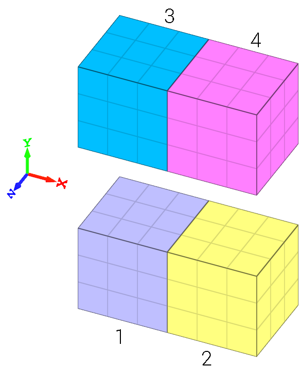
The test consists of 27 CHEX elements in a grid of 3 x 3 x 3, as displayed in Figure 1.
Each element in the grid has unique settings in *BC_MOTION:
1, 1:3, 1:3 - prescribed motions in the X-direction
2, 1:3, 1:3 - prescribed motions in the Y-direction
3, 1:3, 1:3 - prescribed motions in the Z-direction
1:3, 1, 1:3 - prescribed accelerations
1:3, 2, 1:3 - prescribed velocities
1:3, 3, 1:3 - prescribed displacements
1:3, 1:3, 1 - motions defined using a curve
1:3, 1:3, 2 - motions defined using a function
1:3, 1:3, 3 - motions defined using either a curve or a function, with a scale factor defined
For example, the element in position 2, 2, 2 has a prescribed velocity in the Y-direction defined by a function.
The displacement, $d$, velocity, $v$, and acceleration, $a$, are defined so that the displacements of the elements are the same at termination:
$$ d = v \cdot t_{end} = \frac{1}{2} \cdot a \cdot t_{end}^2 $$
The displacements of the elements are checked at termination.
Tests
This benchmark is associated with 1 tests.
Rotational constraints in local coordinate systems
"Optional title"
coid
entype, enid, bc${}_{tr}$, bc${}_{rot}$, csysid${}_{tr}$, csysid${}_{rot}$, $t_{beg}$, $t_{end}$
pmeth${}_1$, direc${}_1$, cid${}_1$, $sf_1$, fid${}_1$
.
pmeth${}_n$, direc${}_n$, cid${}_n$, $sf_n$, fid${}_n$
This test is similair to the test "*BC_MOTION - Rotational constraints in the global coordinate system". In the current test, the rotational constraints are defined in local coordinate systems instead.
Tests
This benchmark is associated with 1 tests.
Rotational constraints in the global coordinate system
"Optional title"
coid
entype, enid, bc${}_{tr}$, bc${}_{rot}$, csysid${}_{tr}$, csysid${}_{rot}$, $t_{beg}$, $t_{end}$
pmeth${}_1$, direc${}_1$, cid${}_1$, $sf_1$, fid${}_1$
.
pmeth${}_n$, direc${}_n$, cid${}_n$, $sf_n$, fid${}_n$
Rotational constraints defined in the global coordinate system are verifed in this test.
Tested parameters: bcrot and csysidrot.
The test consists of 24 CHEX elements positioned as displayed in Figure 1. The three elements in each column has the same rotational constraint. From left to right: 0, X, Y, Z, YZ, ZX, XY, XYZ.
A spin is applied to all elements. The eight elements in each row spin around the same axis but each about its own center of gravity. The rotation point is set in the center of gravity by setting $csysid_{rot} = 0$.
The top row rotates around the Z-axis, the middle row around the Y-axis and the bottom row around the X-axis. At termination the elements that are free to rotate should have rotated $\pi/4$ rad.
The rotations of the elements are checked at termination.
Tests
This benchmark is associated with 1 tests.
Translational constraints in a local coordinate systems
"Optional title"
coid
entype, enid, bc${}_{tr}$, bc${}_{rot}$, csysid${}_{tr}$, csysid${}_{rot}$, $t_{beg}$, $t_{end}$
pmeth${}_1$, direc${}_1$, cid${}_1$, $sf_1$, fid${}_1$
.
pmeth${}_n$, direc${}_n$, cid${}_n$, $sf_n$, fid${}_n$
This test is similair to the test "*BC_MOTION - Translational constraints in the global coordinate system". In the current test, the translational constraints are defined in local coordinate systems instead.
Tests
This benchmark is associated with 1 tests.
Translational constraints in the global coordinate system
"Optional title"
coid
entype, enid, bc${}_{tr}$, bc${}_{rot}$, csysid${}_{tr}$, csysid${}_{rot}$, $t_{beg}$, $t_{end}$
pmeth${}_1$, direc${}_1$, cid${}_1$, $sf_1$, fid${}_1$
.
pmeth${}_n$, direc${}_n$, cid${}_n$, $sf_n$, fid${}_n$
Translational constraints defined in the global coordinate system are verified in this test.
Tested parameter: bctr.
Eight CHEX elements are aligned along the global X-axis as displayed in Figure 1.
A unique translational constraints are imposed on each element. From left to right: 0, X, Y, Z, XY, YZ, ZX, XYZ. A pressure is applied, causing deformation of all elements except the one fixed in XYZ.
At termination, the displacement should be zero in the constrained directions. Displacements in the free directions are calculated based on the applied pressure and bulk modulus of the material.
The displacements of the elements are checked at termination.
Tests
This benchmark is associated with 1 tests.
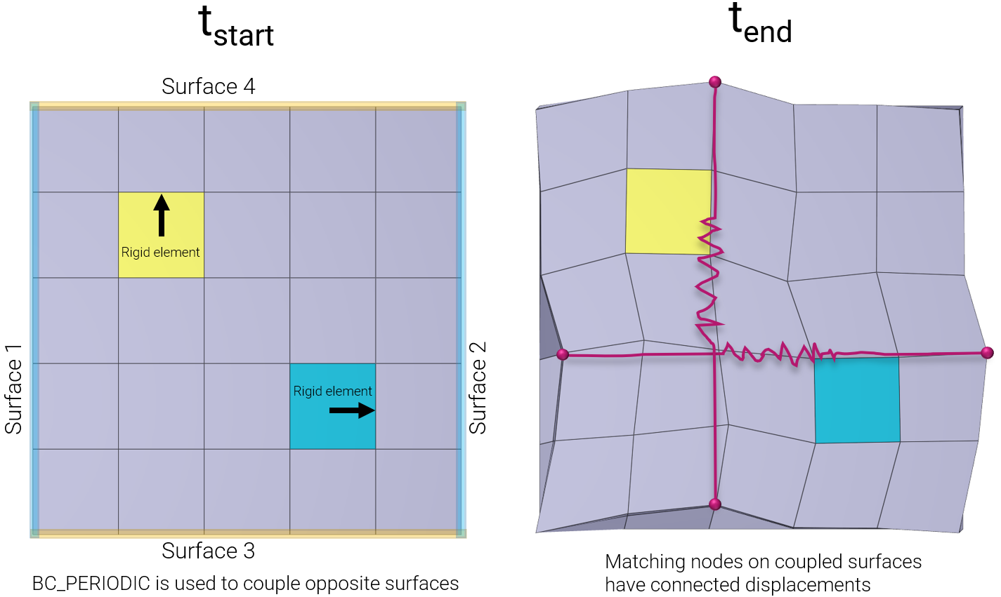
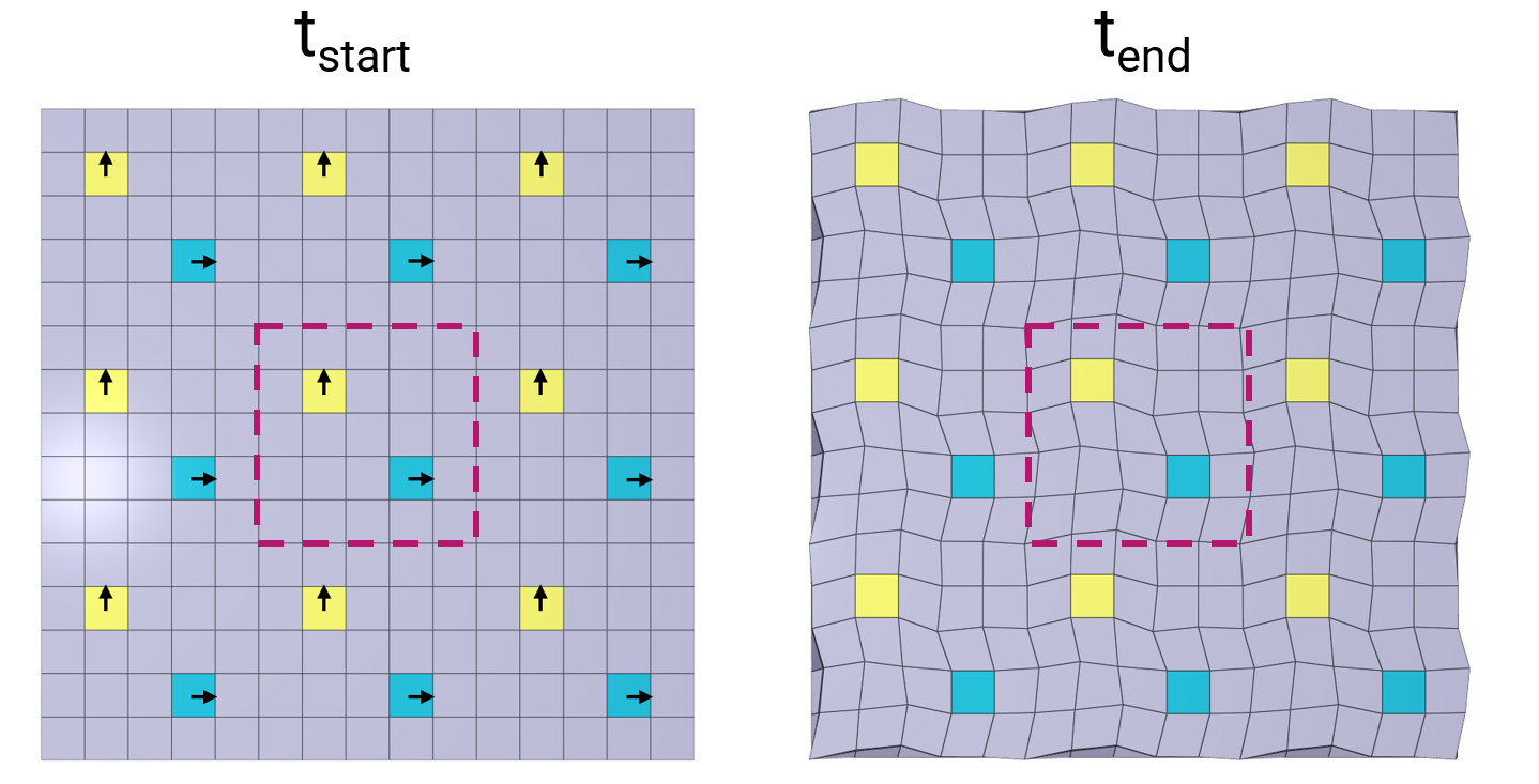
*BC_PERIODIC
Cyclic symmetry
"Optional title"
coid
entype${}_1$, enid${}_1$, entype${}_2$, enid${}_2$
Tested parameters: coid, entype1, enid1, entype2, enid2.
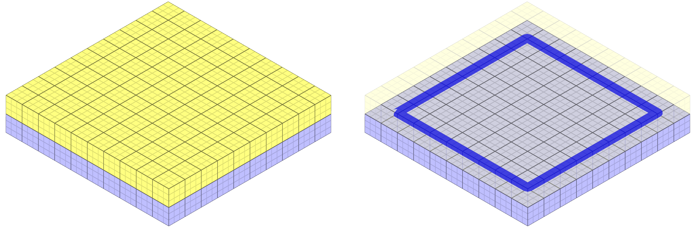
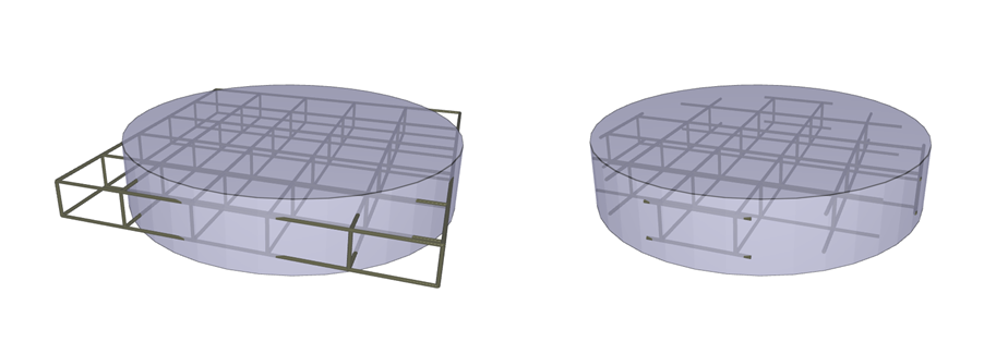
This model tests the command *BC_PERIODIC. Two rigid elements inside a box component is given a prescribed motion in X & Y-direction. The box component consists of a mesh of 5x5x2 elements. Motion in Z-direction is restricted for the entire model. The bottom surface is completely fixed. To apply cyclic symmetry to the model, periodic boundary conditions are used to couple surface 1 & 2, and surface 3 & 4. The corresponding nodes for the coupled surfaces experience equivalent displacements. See Figure 1.
A larger model displaying the repetitive pattern is illustrated in Figure 2.
Node displacements are checked for version control.
Tests
This benchmark is associated with 1 tests.
*BC_SYMMETRY
Rigid wall
plane, csysid${}_1$, csysid${}_2$, csysid${}_3$, $tol$
This model tests the command *BC_SYMMETRY. The test consists of six CHEX elements, all located at a distance from the symmetry planes defined in the global coordinate system. The elements are given a prescribed velocity in the -Z, +Z, -Y, +Y, -X, +X directions. None of the elements should pass through any of the axes of the symmetry planes. See Figure 1.
X, Y and Z coordinates of the elements are checked for version control.
Tests
This benchmark is associated with 1 tests.
Symmetry in local coordinate systems
plane, csysid${}_1$, csysid${}_2$, csysid${}_3$, $tol$
Symmetry and tolerance defined in local coordinate systems are verified in this test.
Tested parameters: csysid1, csysid2, csysid3, tol
An element is defined by the coordinates ($d$, $d$, $d$) and ($L+d$, $L+d$, $L+d$), where $L$ is the element side length and $d$ is an offset distance. Three local coordinate systems are defined as displayed in Figure 1. and described in Table 1. Symmetry conditions are defined in these local coordinate systems.
| Local coordinate system ID | Origin | Local x-axis [X, Y, Z] |
|---|---|---|
| 11 | 0, L/2, L/2 | 1, 0, 0 |
| 12 | L/2, 0, L/2 | 0, 1, 0 |
| 13 | L/2, L/2, 0 | 0, 0, 1 |
Prescribed motions are imposed on the three surfaces opposite the surfaces affected by the symmetry.
Two tests are done. In the first test, the tolerance is greater than $d$, meaning that symmetry will be active, and the element expands because of the prescribed motions. In the second test, the tolerace is smallar than $d$, meaning that symmetry conditions are not active, and the cube will translate instead of expanding.
The displacements of the nodes initially located at ($d$, $d$, $d$) and ($L+d$, $L+d$, $L+d$) are checked at termination.
Tests
This benchmark is associated with 2 tests.
Symmetry in the global coordinate system
plane, csysid${}_1$, csysid${}_2$, csysid${}_3$, $tol$
Symmetry options and tolerance defined in the global coordinate system are verified in this test.
Tested parameters: $plane$ and $tol$.
The test consists of a CHEX element defined by the coordinates ($d$, $d$, $d$) and ($L+d$, $L+d$, $L+d$), where $L$ is the element side length and $d$ is an offset distance. Prescribed displacements are imposed on the surfaces opposite the symmetry surfaces. The displacements are in the normal directions of the surfaces.
A total of 16 configurations of the model are run and these can be divided into two sets. All symmetry options (0, X, Y, Z, XY, YZ, ZX, XYZ) are tested for both sets. In one of the sets, the tolerance is greater than the offset distance and in the other set it is not, meaning that the symmetry is not activated.
At termination, the displacement of the surfaces affected by the symmetry should be equal to zero. The displacement of free surfaces should be equal to the prescribed displacement.
The displacements of the nodes initially located at ($d$, $d$, $d$) and ($L+d$, $L+d$, $L+d$) are checked at termination.
Tests
This benchmark is associated with 16 tests.
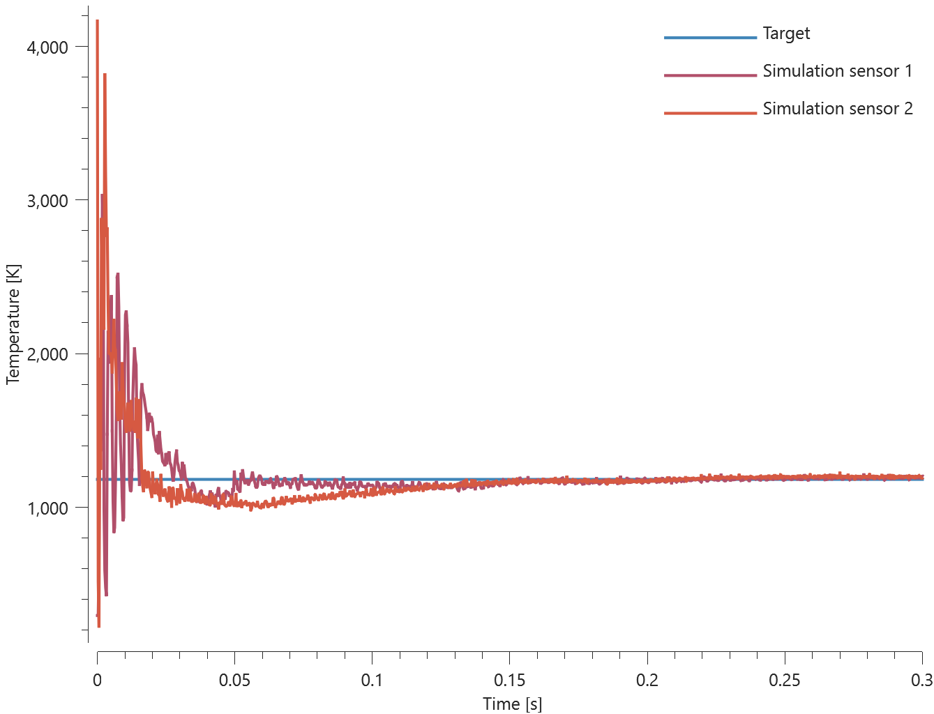
*BC_TELEPORT
Displacements and velocities in the global coordinate system
"Optional title"
coid
entype, enid, csysid, trig, multiple, velocity
$\Delta_x$, $\Delta_y$, $\Delta_z$, $\theta_x$, $\theta_y$, $\theta_z$, $\Delta v_x$, $\Delta v_y$, $\Delta v_z$
Teleportation displacements and velocities in the global coordinate system are verfied in this test.
Tested parameters: trig, $\Delta_x$, $\Delta_y$, $\Delta_z$, $\Delta v_x$, $\Delta v_y$, $\Delta v_z$.
A CHEX element is given the initial velocity $v_{0,x}$, $v_{0,y} = 2 v_{0,x}$ and $v_{0,z} = 3 v_{0,x}$.
Teleportation displacements are defined in the global coordinate system as:
$\Delta_x = -v_{0,x}\cdot trig$, $\Delta_y = -v_{0,y}\cdot trig$, $\Delta_z = -v_{0,z}\cdot trig$
Parameter $trig$ is set to half the termination time.
Teleportation velocities are defined as:
$\Delta v_x = -v_{0,x}$, $\Delta v_y = -v_{0,y}$ and $\Delta v_z = -v_{0,z}$.
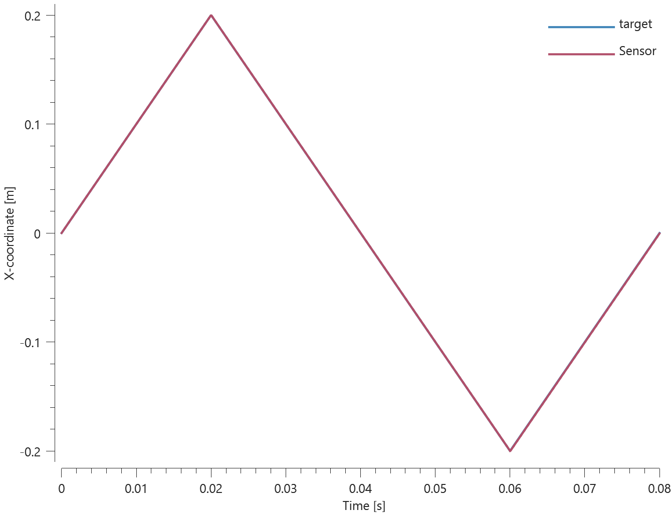
A sensor is located in the center of the element, which coincides with the origin of the global coordinate system at initiation.
Coordinates of the sensor at teleportation should be:
$v_{0,x}\cdot trig$, $v_{0,y}\cdot trig$ and $v_{0,z}\cdot trig$ in the X-, Y- and Z-direction.
Coordinates of the sensor at termination should be:
$-\Delta v_x\cdot (term-trig)$, $-\Delta v_y\cdot (term-trig)$ and $-\Delta v_z\cdot (term-trig)$ in X-, Y- and Z-direction.
Parameter $term$ is the termination time.
Sensor coordinates vs. time is presented in Figure 1. together with target curves.
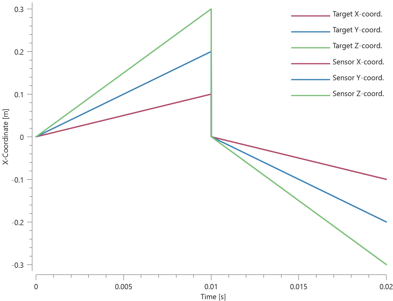
Max, min and average values of sensor coordinates are checked.
Tests
This benchmark is associated with 1 tests.
Multiple teleportations using trigger function
"Optional title"
coid
entype, enid, csysid, trig, multiple, velocity
$\Delta_x$, $\Delta_y$, $\Delta_z$, $\theta_x$, $\theta_y$, $\theta_z$, $\Delta v_x$, $\Delta v_y$, $\Delta v_z$
Multiple teleportations using a trigger function is verfied in this test.
Tested parameters: $trig$, $\Delta_x$, $\Delta_y$, $\Delta_z$, $multiple$ and $velocity$.
A CHEX element is given the initial velocity $v_{0,x}$, $v_{0,y} = 2 v_{0,x}$ and $v_{0,z} = 3 v_{0,x}$.
A sensor (with id = 1) is defined at the center of the element, which coincides with the origin of the global coordinate system at initiation.
A trigger function is defiend as:
$$ \sqrt{xs(1)^2 + ys(1)^2 + zs(1)^2} - disp_{max} $$
The first term corresponds to the sensor displacement and $disp_{max}$ is the displacement at which teleportation is to occur, defined as:
$$ disp_{max} = trig\cdot \sqrt{v_{0,x}^2+v_{0,y}^2+v_{0,z}^2} $$
Parameter $trig$ is set to a third of the termination time.
Teleportation displacements are defined as $\Delta_x = -v_{0,x} \cdot trig$, $\Delta_y = -v_{0,y} \cdot trig$, $\Delta_z = -v_{0,z} \cdot trig$, meaning that the element is teleported to its initial position, and the velocities are defined to continue after teleportation.
This configuration should generate two teleportations, and the sensor coordinates at termination should be:
$trig\cdot v_{0,x}$, $trig\cdot v_{0,y}$ and $trig\cdot v_{0,z}$ in the X-, Y- and Z-direction.
Sensor coordinates vs. time is presented in Figure 1. together with target curves.
Max, min and average values of sensor coordinates are checked.
Tests
This benchmark is associated with 1 tests.
Rotations in a local coordinate system
"Optional title"
coid
entype, enid, csysid, trig, multiple, velocity
$\Delta_x$, $\Delta_y$, $\Delta_z$, $\theta_x$, $\theta_y$, $\theta_z$, $\Delta v_x$, $\Delta v_y$, $\Delta v_z$
Teleportation rotations in a local coordinate system are verified in this test.
Tested parameters: $trig$ and $\theta_z$.
Two CHEX elements are defined in a local coordinate system, which at initiation coincides with the global coordinate system. A sensor (id = 1) is defined at the origin of the local coordinate system. The elements are given an initial velocity $v_0$ in the local X-direction.
A trigger function for teleportation is defined as:
$$ abs(xs(1)) - X_{max} $$
$abs(xs(1))$ corresponds to the absolute value of the sensor X-coordinate and $X_{max}$ is the displacement at which teleportation should occur.
Teleportation rotation is defined as $\theta_z = \pi$, and the velocity is defined to continue after the teleportation. This means that after rotation, the local X-direction (which is the elements velocity vector) changes direction and is now opposite the global X-direction.
A second teleportation occurs once the sensor X-displacement reaches $-X_{max}$. After this teleportation, the local X-axis coincides with the global X-axis again.
Sensor X-coordinate vs. time is presented in Figure 1. together with a target curve.
Max, min and average value of sensor X-coordinate is checked.
Tests
This benchmark is associated with 1 tests.
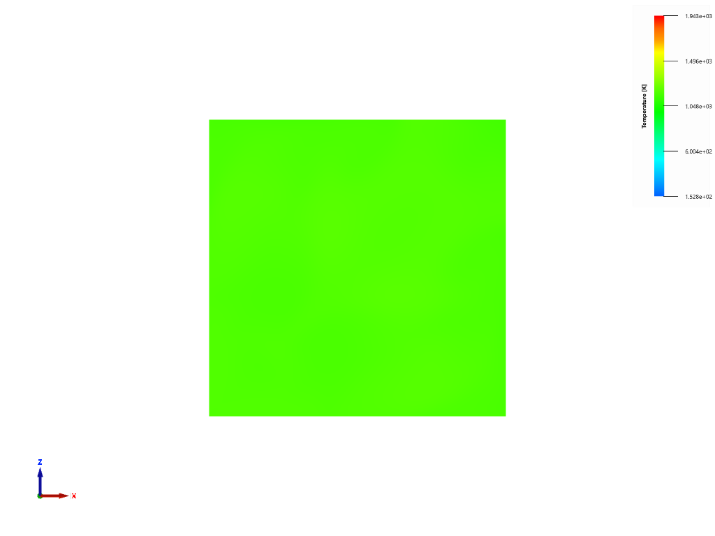
*BC_TEMPERATURE
All features
"Optional title"
entype, enid, cid, $sf$, $t_{beg}$, $t_{end}$
All features of *BC_TEMPERATURE are verified in this test.
Tested parameters: $cid$, $sf$, $t_{beg}$ and $t_{end}$.
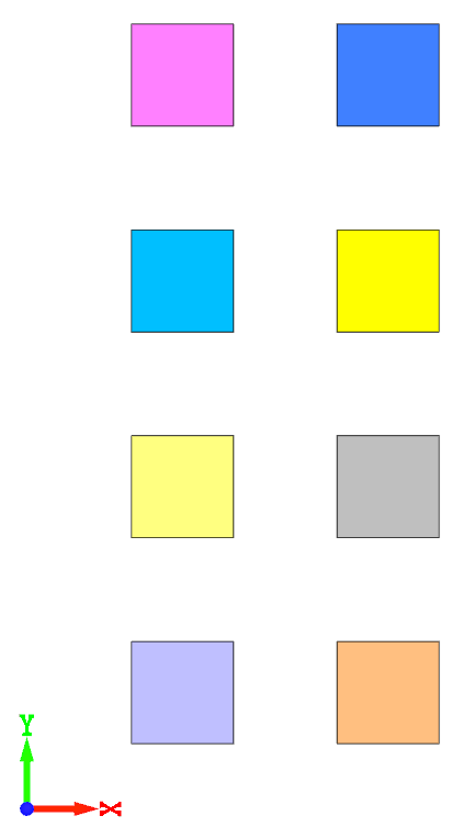
Eight CHEX elements are positioned as displayed in Figure 1. The temperature of the four elements in the left column is controlled by a curve while the temperature of the elements in the right column is controlled by a function.
The curve is defined as:
| Time | Temperature |
|---|---|
| 0 | 0 |
| $t_{end}$ | $T_{max}$ |
The function is defined as:
$$ T(X, t) = \left(\frac{X - X_{min}}{X_{max} - X_{min}}\right) \cdot \left(\frac{t}{t_{end}}\right) \cdot T_{max} $$
$t_{end}$ is the termination time and $T_{max}$ is the maximum temperature. $X$ corresponds to the X-coordinate and $t$ the current time in the simulation. $X_{min}$ and $X_{max}$ are minimum and maximum X-coordinates of the elements in the right column.
The temperatures in the two elements at the top row are just controlled by the curve and function. In the second row, a scale factor of 0.5 is used. Activation and deactivation times are used in the third and forth row respectively.
Maximum and average temperature are checked in the elements.
Tests
This benchmark is associated with 1 tests.
One-dimensional heat conduction
"Optional title"
entype, enid, cid, $sf$, $t_{beg}$, $t_{end}$
One-dimensional heat conduction is verified in this test.
Tested parameters: $entype$, $enid$ and $cid$.
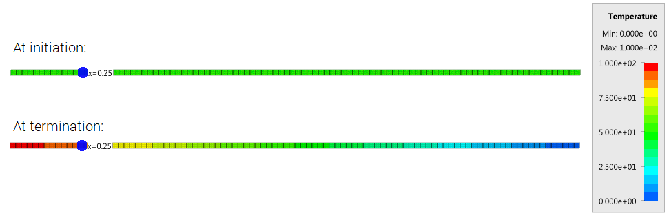
Prescribed temperatures are imposed at the ends of a rod with an initial uniform temperature, causing the temperature along the rod to change due to conduction. The initial and final temperature in a sensor located at the blue mark in Figure 1. is compared to analytical results.
Temperature at initiation and termination is checked.
Tests
This benchmark is associated with 1 tests.
*BOLT_FAILURE
Failure criterias
"Optional title"
coid
pid, tid, $T_{fail}$, $S_{fail}$, $W_{fail}$
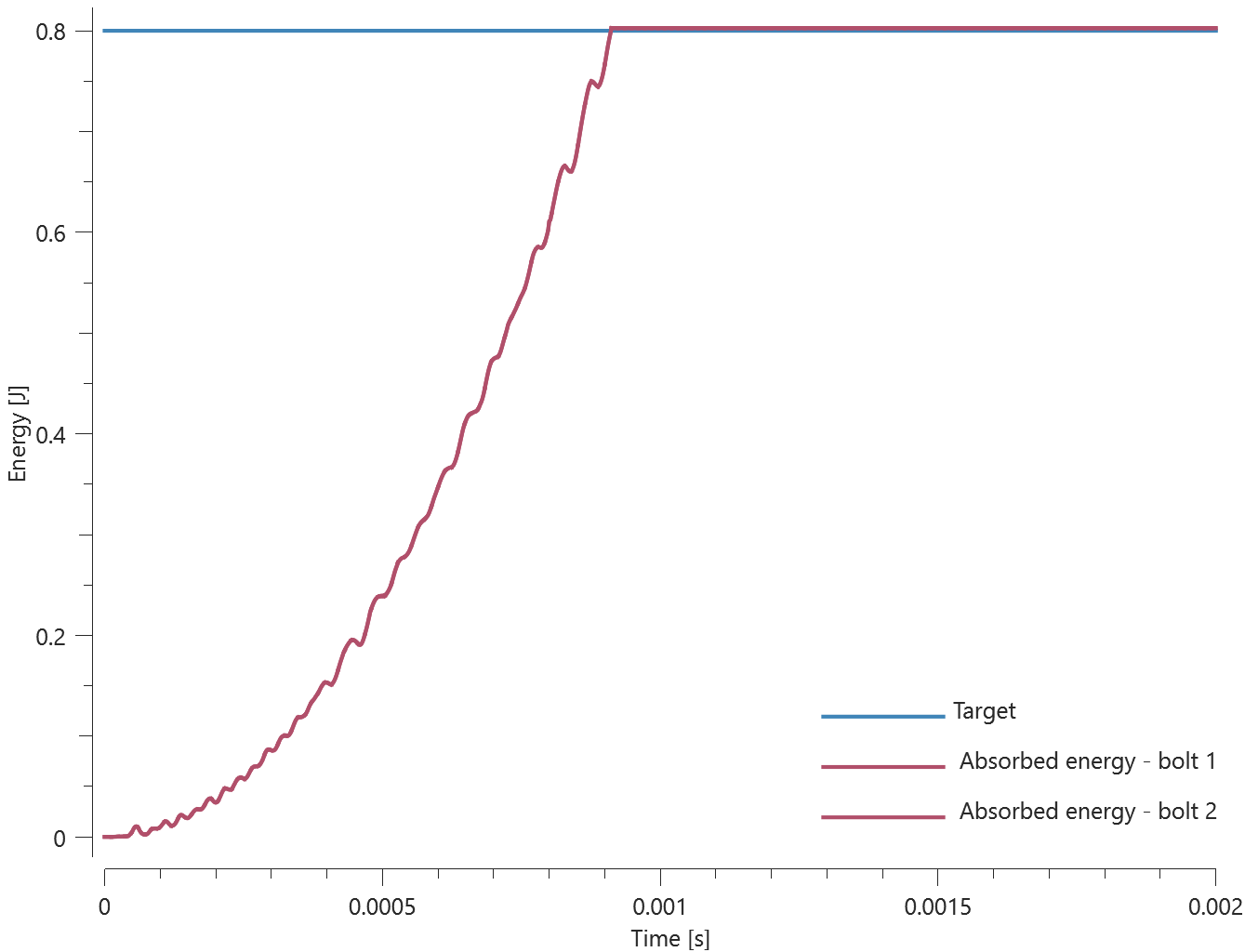
This tests the *BOLT_FAILURE command. In this benchmark, the bolt failure functionality is tested for two bolts. The bolts are modelled by *COMPONENT_BOLT and the test model is presented in Figure 1.
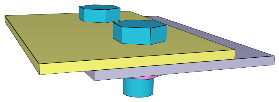
The bolts are prestressed up until failure. The test is done twice with different parameters set for $T_{fail}$, $S_{fail}$ and $W_{fail}$. This is to ensure that the criteria for the damage parameter, $D$, is fulfilled both by reaching the force limit and the energy absorbed limit. Once $D = 1$ the bolts are eroded, see Figure 2.
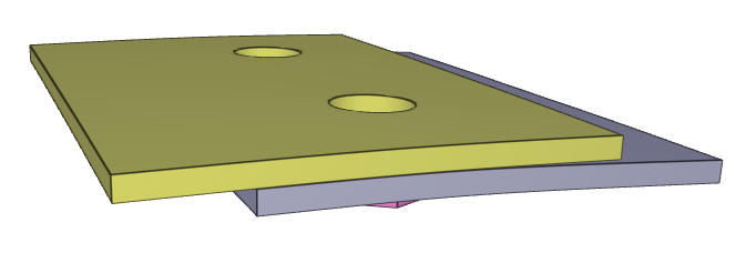
For both the tests the maximum value of the damage parameter is checked. For the test were the minimum abosorbed energy prior to failure is checked, the maximum absorbed energy is also checked.
Tests
This benchmark is associated with 2 tests.
*CFD_BLAST_1D
Sensitivity study
"Optional title"
coid, Stype, sid_gas, sid_exp
m_exp, R_exp, R_max, R_term, n_cells, n_dump
t_det, R_det, r_thres, i_write, dt_cfl
This is a copy of the senasativity study of the *CFD_BLAST_1D command in the command manual. A 1kg spherical TNT charge detonated in free air. The incident pressure and incident impulse is then compared to the Kingery-Bulmash equations.
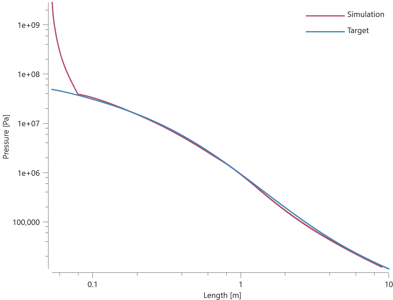
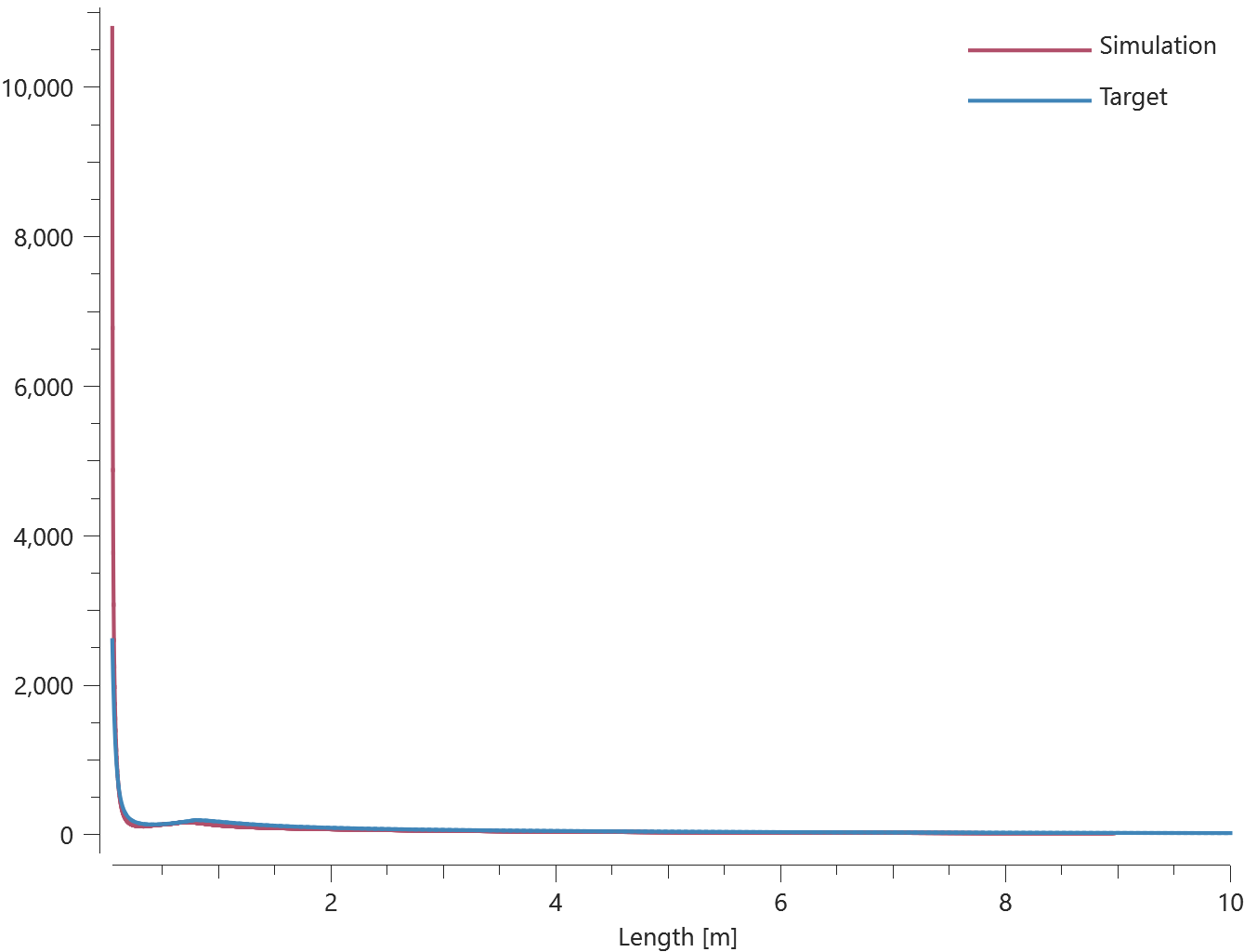
Checks for incident pressure and incident impulse are done in 11 sensors placed in an interval 0.3-9 m from the detonation.
Tests
This benchmark is associated with 1 tests.
*CFD_DETONATION
Detonation radius
"Optional title"
coid
$x_d$, $y_d$, $z_d$, $t_d$, $R$, path
Tested parameters: $R$.
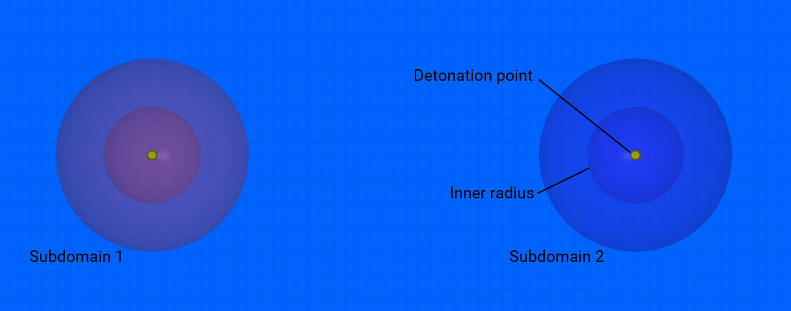
This model tests the parameter $R$ in *CFD_DETONATION, which is used to limit the distance the detonation front is allowed to propagate through programmed burn. The test consists of two spherical CFD HE subdomains both with an inner radius of 10 mm and outer radius of 20 mm. A detonation point is set in the centre of each sphere. One of the subdomain's detonation radius is limited to its inner radius by setting $R = 0.01$. It is tested that only the subdomain without the radius limitation is triggered from the detonation.
The test setup can be seen in Figure 1.
Undetonated energy vs. time can be seen in Figure 2.
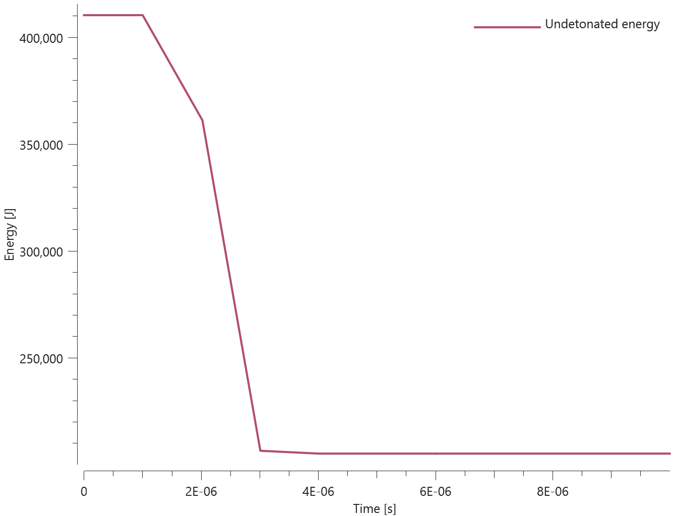
First and last value of undetonated energy is checked for version control.
Tests
This benchmark is associated with 1 tests.
FE to CFD switch
"Optional title"
coid
$x_d$, $y_d$, $z_d$, $t_d$, $R$, path, pid
This is a verification test from the command manual for *CFD_DETONATION. A sphere is given an initial velocity towards a cylinder of explosives. The explosive is modelled with finite elements, but when the sphere hits the explosive and the detonation criteria is met the explosive will switch to CFD cells.
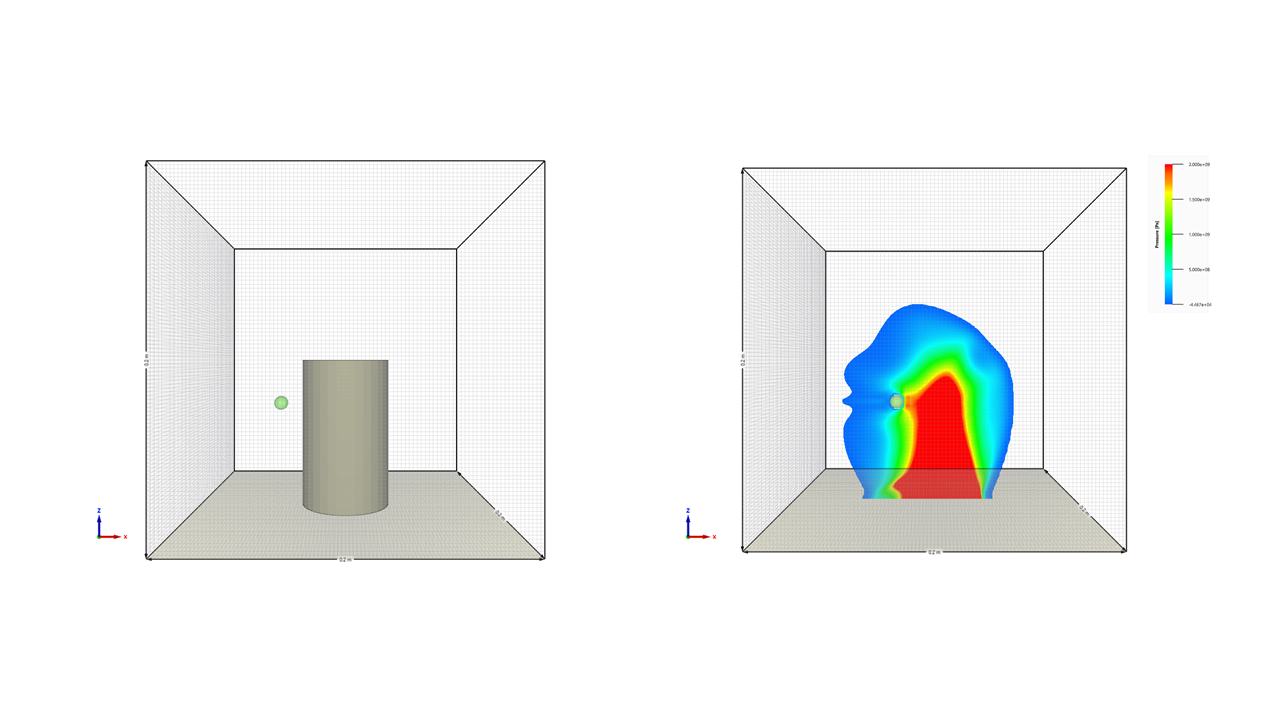
Maximum, first and last value of pressure in a sensor in the middle of the grid is done for verison control.
*CFD_DOMAIN
Airblast propagation
"Optional title"
coid
entype, enid, $\Delta$, air, geo_update, xsmooth, blocking_update
$x_0$, $y_0$, $z_0$, $x_1$, $y_1$, $z_1$
bc${}_{x0}$, bc${}_{y0}$, bc${}_{z0}$, bc${}_{x1}$, bc${}_{y1}$, bc${}_{z1}$
$t_{end}$
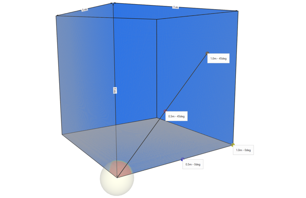
This model tests airblast propagation for the CFD solver. A hemi-spherical blast modeled with quarter symmetry is detonated. To determine sphericity of the charge at close range, sensors are placed at 0° and 45° angle, measuring the time the blast wave arrives. This is done at two distances, 0.5 and 1.0 meters from the detonation point. Also, incident pressure is being measured. The test setup can be seen in Figure 1.
The configuration is a 0.853493 g TNT charge. Considering half shape and quarter symmerty, the size of the charge would be equal to a charge in free air of:
$$ m_{free \ air} = 0.853493 \cdot 8 = 6.827944 \ kg $$
And due to energy absorbed by the ground, a correction factor of 1.8 is being used:
$$ m_{hemisphere} = \frac{m_{free \ air}}{1.8} $$
Which for this configuration will be a charge of:
$$ m_{hemisphere} = \frac{6.827944}{1.8} = 3.8 \ kg $$
The results are compared with analytical values from Kingery-Bulmash.
| Kingery-Bulmash Blast Parameter Calculator: TNT, 3.8kg, 0.5m: | |
|---|---|
| TNT Weight for Pressure (kg): | 3.80 |
| Incident Pressure (kPa): | 9325.38 |
| Reflected Pressure (kPa): | 86856.97 |
| Time of Arrival (ms): | 0.11 |
| Shock Front Velocity (m/s): | 2950.51 |
| TNT Weight for Impulse (kg): | 3.80 |
| Incident Impulse (kPa-ms): | 316.38 |
| Reflected Impulse (kPa-ms): | 7408.46 |
| Positive Phase Duration (ms): | 0.35 |
| Kingery-Bulmash Blast Parameter Calculator: TNT, 3.8kg, 1.0m: | |
|---|---|
| TNT Weight for Pressure (kg): | 3.80 |
| Incident Pressure (kPa): | 3222.15 |
| Reflected Pressure (kPa): | 23926.54 |
| Time of Arrival (ms): | 0.34 |
| Shock Front Velocity (m/s): | 1791.97 |
| TNT Weight for Impulse (kg): | 3.80 |
| Incident Impulse (kPa-ms): | 273.25 |
| Reflected Impulse (kPa-ms): | 2567.19 |
| Positive Phase Duration (ms): | 0.68 |
Incident pressure vs. time can be seen in Figure 2.
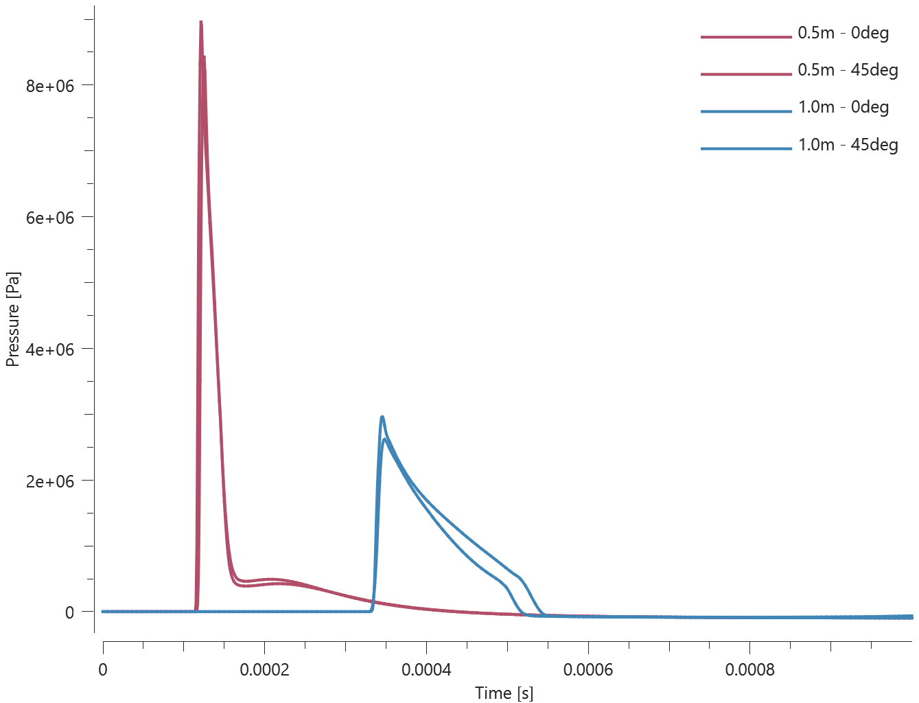
Maximum value of incident pressure and time of arrival at the sensors is checked for version control.
Tests
This benchmark is associated with 1 tests.
Airblast propagation with restart
"Optional title"
coid
entype, enid, $\Delta$, air, geo_update, xsmooth, blocking_update
$x_0$, $y_0$, $z_0$, $x_1$, $y_1$, $z_1$
bc${}_{x0}$, bc${}_{y0}$, bc${}_{z0}$, bc${}_{x1}$, bc${}_{y1}$, bc${}_{z1}$
$t_{end}$
This test is similar to the test "*CFD_DOMAIN - Airblast propagation". The difference is that it is being run in two steps.
In step 1, Time and incident pressure is being measured for the closest sensors at $0.5 \ m$ range. The simulation is then stopped.
In step 2, the simulation continues from the output of step 1. Time and incident pressure is beging measured for the sensors at $1.0 \ m$ range.
The expected outcome is to get the same results as the test "*CFD_DOMAIN - Airblast propagation".
Tests
This benchmark is associated with 2 tests.
CFD-FE-SPH Coupling
"Optional title"
coid
entype, enid, $\Delta$, air, geo_update, xsmooth, blocking_update
$x_0$, $y_0$, $z_0$, $x_1$, $y_1$, $z_1$
bc${}_{x0}$, bc${}_{y0}$, bc${}_{z0}$, bc${}_{x1}$, bc${}_{y1}$, bc${}_{z1}$
$t_{end}$
This model tests that the CFD coupling correctly handles the interaction with Finite Elements and SPH particles at the same time.
The test setup consists of two geometrically identical plates on each side of a spherical charge in the CFD-Domain. Quarter symmetry is used. One is modeled with Finite Elements and the other with SPH Particles. The response should be the same for both methods.
The test setup can be seen in Figure 1.
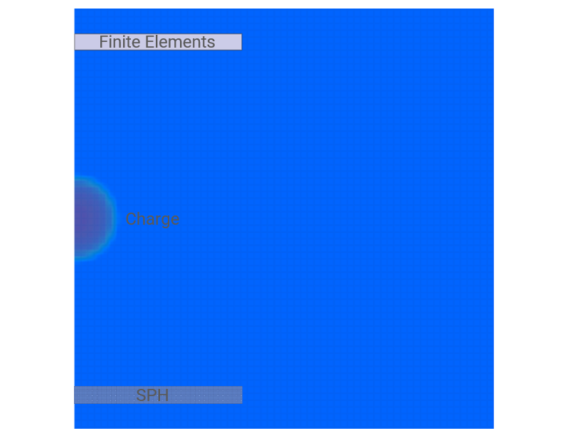
The velocity of the plates in Z-direction is measured.
Velocity vs. time can be seen in Figure 2.
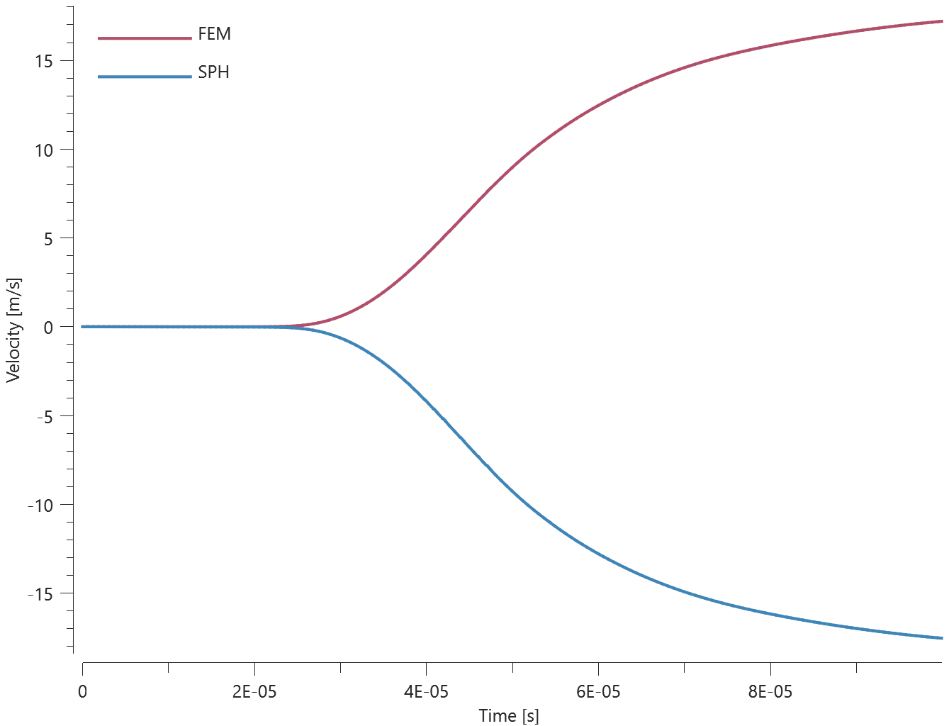
Last and average velocity is checked for version control.
Tests
This benchmark is associated with 1 tests.
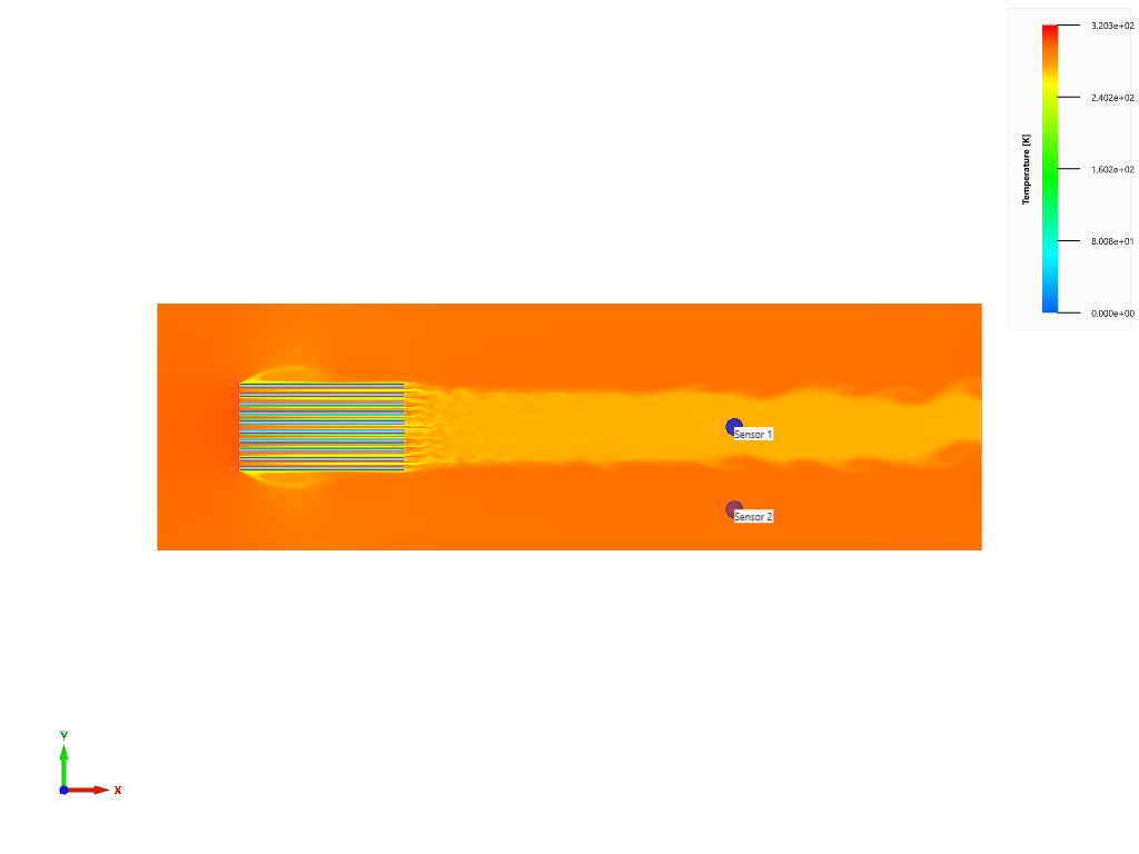
*CFD_GAS
CFD_GAS - Gas properties mix
"Optional title"
sid
type, gid,
$\rho$, $\gamma$, $e_0$, $C_v$, $b$
This model tests the CFD solver when gases with different thermal proeperties mixes. *CFD_GAS is used to create a user defined gas. The gas is contained in a sphere geometry, before being released in a CFD domain containing air. After the gases are mixed together, the gas temperature and density are measured and compared to an analytical calculated result. This tests the parameters $\rho$, $\gamma$, $e_0$ and $C_v$.
The model at initiation can be seen in Figure 1. The model have been sliced at the center of the sphere with gas and shows both the sensors.
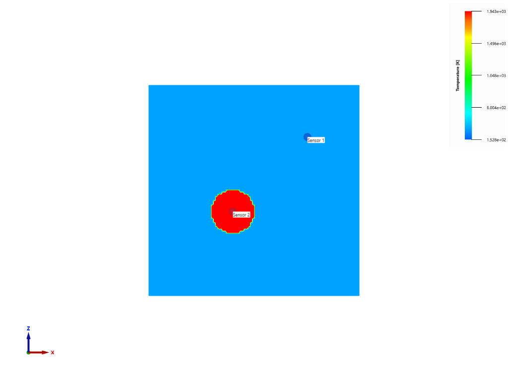
The final state of the simulation can be seen in Figure 2.
In Figure 3 and Figure 4 the reults from the simulation are shown.
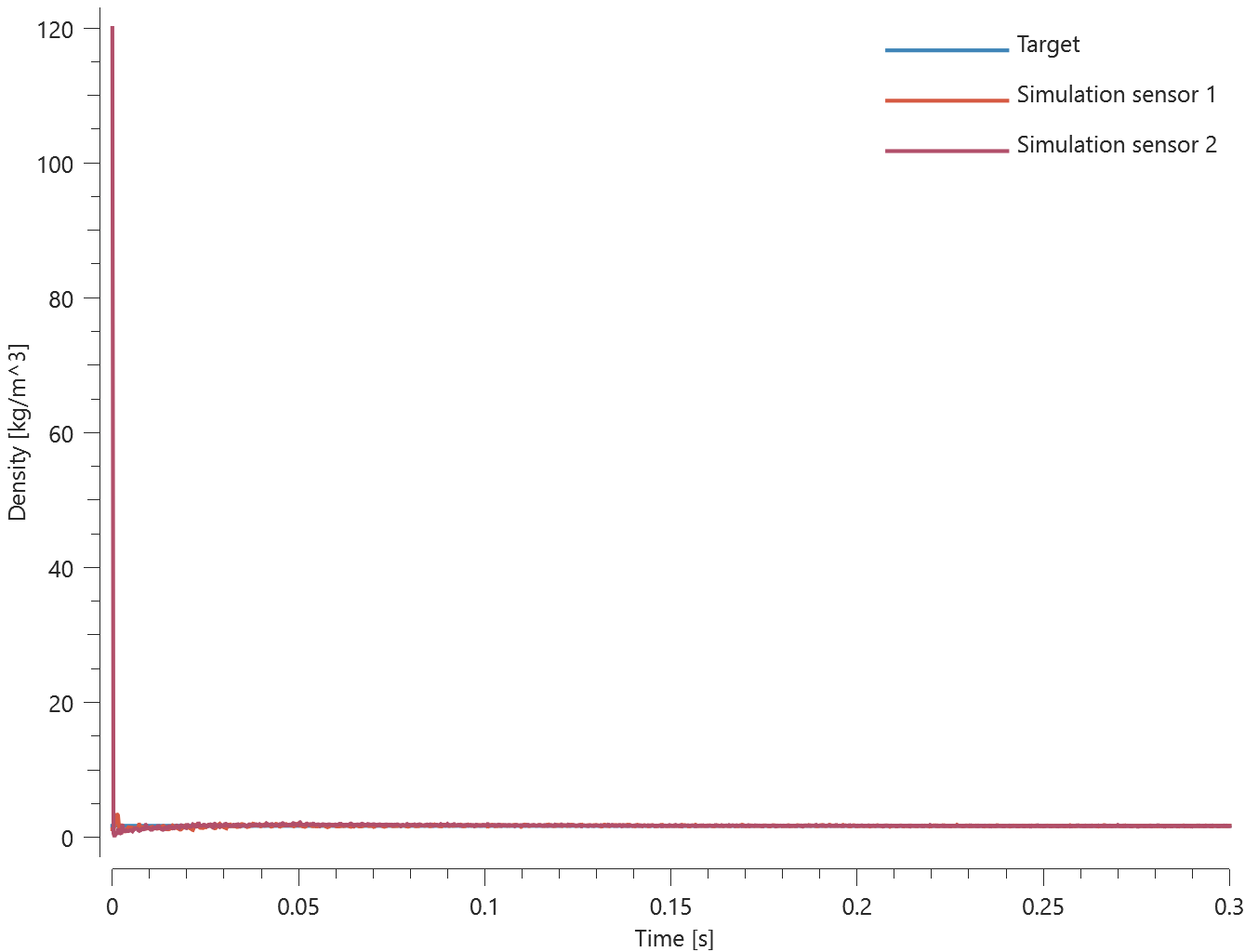
The last value of the temperature and the gas density is checked at the two sensors.
Tests
This benchmark is associated with 1 tests.
*CFD_STRUCTURE_INTERACTION
Cooling
"Optional title"
coid, output, $\delta_{off}$
entype, enid, itype, $C_1$, $C_2$
fid$_{thermal}$
This model tests the cooling effectes of a solild FE structure coupled with the CFD domain.
A wind tunnel is set up using *CFD_WIND_TUNNEL. Inside 10 solid FE bars are placed and locked in space. The structures are coupled with the CFD doamin using *CFD_STRUCTURE_INTERACTION. A function for gas cooling is then applied for the bars, all gas that interact with the structure should therefore be cooled.
Version control is done with one sensor placed behind the bars and one below them. The sensor below the bars should have the the same temperature during the whole simulation, while the one behind should have a lowered temperature due to the cooling.
*CFD_WIND_TUNNEL
Normal shock stagnation state
"Optional title"
fid$_{v}$
In this benchmark the *CFD_WIND_TUNNEL command is tested. A rigid plate is created in a CFD domain. The domain is then converted to a wind tunnel using *CFD_WIND_TUNNEL. The model at initiation can be seen in Figure 1.

Once the simulation reaches normal shock stagnation state, see Figure 2, values for temperature, gas density and pressure are obtained at a sensor 2 mm from the plate surface.

Results from the simulation at the sensor can be seen in Figures 3 - 5


Local deviations from the analytical result are due to the shock viscosity.
The last values for density, temperature and pressure from the simulation are compared to analytical results.
Tests
This benchmark is associated with 1 tests.
*CHANGE_P-ORDER
Cantilever beams
"Optional title"
entype, enid, order, gid
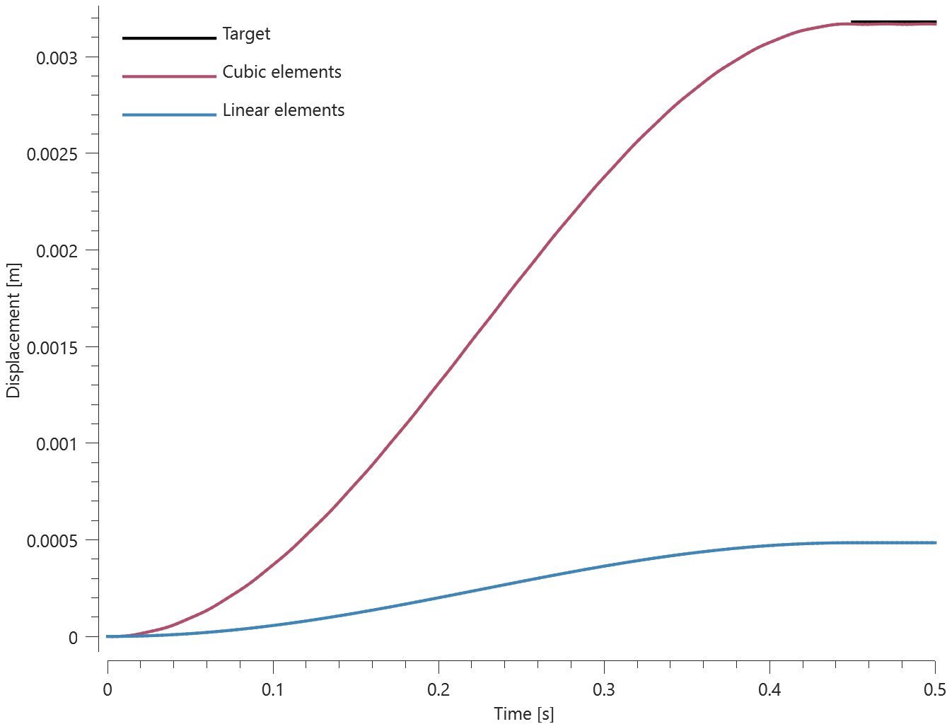
This test shows that higher order elements are superior to linear elements in the case of bending.
Tested parameters: $entype$, $enid$ and $order$.
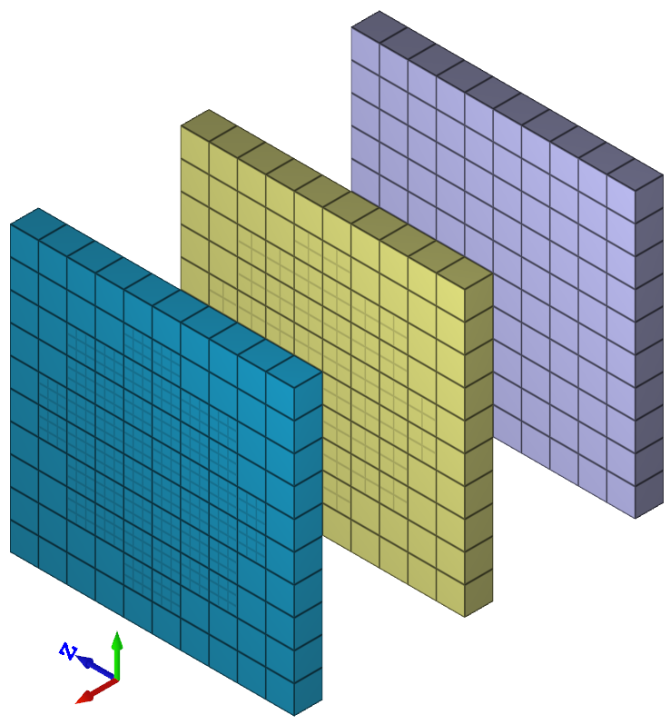
Two cantilever beams are subjected to a transverse point load at the unconstrained end. One of the beams is modeled with five LHEX elements and the other with five CHEX elements, as visible in Figure 1.

The displacements of the ends vs. time from the simulation are plotted in Figure 2 together with an analytical value of max deflection obtained from Euler-Bernoulli beam theory.
Tests
This benchmark is associated with 1 tests.
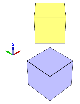
Domain of higher order elements
"Optional title"
entype, enid, order, gid
Conversion to higher order elements within a specified geometry is verified in this test.
Tested parameters: $entype$, $enid$, $order$ and $gid$.
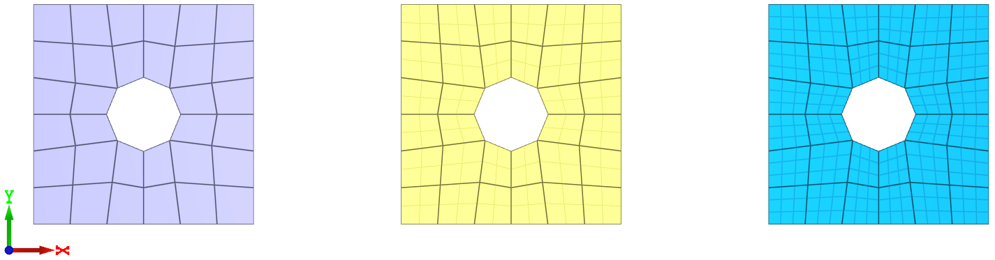
Three square plates modeled with LHEX elements are positioned as displayed in Figure 1. A geometry (*GEOMETRY_PIPE) is defined with its axial direction aligned with the center of the plates. The diameter of the geometry is smaller than the side length of the plates, meaning that only a part of the plates is inside the geometry. Elements within the geometry are converted to the higher order elements in two of the plates.
The coordinates of a node in each plate are checked.
Tests
This benchmark is associated with 1 tests.
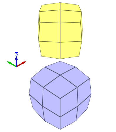
Higher order elements
"Optional title"
entype, enid, order, gid
Conversion from linear elements to higher order elements with *CHANGE_P-ORDER is verified in this test.
Tested parameters: $entype$, $enid$ and $order$.
Three plates meshed with LHEX elements are used in this test. Each plate is assigned a unique polynomial order (1,2 or 3) in *CHANGE_P-ORDER. The elements in two of the plates are therefore converted into higher order elements as visible in Figure 1.
The coordinates of a node in each plate are checked.
Tests
This benchmark is associated with 1 tests.
*CHANGE_PART_ID
Elements inside a geometry
"Optional title"
coid
pid${}_{from}$, pid${}_{to}$, gid
Tested parameters: coid, pidfrom, pidto, gid.
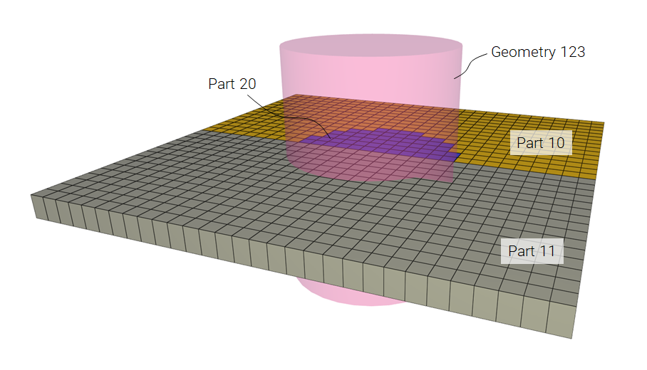
The model tests the command *CHANGE_PART_ID. The test consists of two parts and a geometry. With the use of the command *CHANGE_PART_ID the elements of Part 10 that are inside Geometry 123 will be moved to Part 20. See Figure 1.
The physical mass of part 10, 11 & 20 is checked for version control.
Tests
This benchmark is associated with 1 tests.
Included files
"Optional title"
coid
pid${}_{from}$, pid${}_{to}$, gid
Tested parameters: coid, pidfrom, pidto, gid
The model tests that the command *CHANGE_PART_ID is functioning within included files when using offsets to part ID:s. The test is similar to the test "*INCLUDE - Offset" and should give the same result.
Targets:
-First cube should rotate 1 lap about X-axis.
-Second cube should move downwards 1 m in Z-direction.
Tests
This benchmark is associated with 1 tests.
*COMPONENT_BOLT
Defined in global and local coordinate systems
"Optional title"
coid, pid${}_1$, pid${}_2$, pid${}_3$, pid${}_4$, csysid, tid
$D$, $L$, $h$, $t$
Dimensions and positioning of bolts defined with *COMPONENT_BOLT are verified in this test.
Tested parameters: $pid_1$, $pid_2$, $pid_3$, $pid_4$, $csysid$, $D$, $L$, $h$ and $t$.
Two bolts are created using *COMPONENT_BOLT. One is created in the global coordinate system and the other in a local coordinate system. Both the origin and the axes in the local coordinate system differs from the global system, as visible in Figure 1.
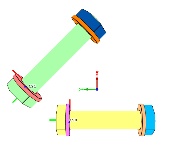
Coordinates for a number of nodes are checked.
Tests
This benchmark is associated with 1 tests.
Positioning with table
"Optional title"
coid, pid${}_1$, pid${}_2$, pid${}_3$, pid${}_4$, csysid, tid
$D$, $L$, $h$, $t$
Positioning of bolts with the command *TABLE is verified in this test.
Tested parameters: $pid_1$, $pid_2$, $pid_3$, $pid_4$, $tid$, $D$, $L$, $h$ and $t$.
A number of bolts are positioned as displayed in Figure 1. by using the command *TABLE.
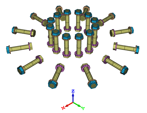
Coordinates for some of the nodes are checked.
Tests
This benchmark is associated with 1 tests.
*COMPONENT_BOX
Defined in global and local coordinate systems
"Optional title"
coid, pid, N${}_x$, N${}_y$, N${}_z$, csysid
$x_1$, $y_1$, $z_1$, $x_2$, $y_2$, $z_2$
Dimensions and positioning of boxes defined with *COMPONENT_BOX are verified in this test.
Tested parameters: $pid$, $N_x$, $N_y$, $N_z$, $csysid$, $x_1$, $y_1$, $z_1$, $x_2$, $y_2$ and $z_2$.
Two boxes are created using *COMPONENT_BOX. One is created in the global coordinate system and the other one in a local coordinate system. Both the origin and the axes in the local coordinate system differs from the global system, as visible in Figure 1.
Coordinates for a number of nodes are checked.
Tests
This benchmark is associated with 1 tests.
*COMPONENT_BOX_IRREGULAR
Defined in global and local coordinate systems
"Optional title"
coid, pid, N${}_1$, N${}_2$, N${}_3$, csysid
$x_1$, $y_1$, $z_1$, $x_2$, $y_2$, $z_2$
$x_3$, $y_3$, $z_3$, $x_4$, $y_4$, $z_4$
$x_5$, $y_5$, $z_5$, $x_6$, $y_6$, $z_6$
$x_7$, $y_7$, $z_7$, $x_8$, $y_8$, $z_8$
id1, $x_{id1}$, $y_{id1}$, $z_{id1}$, id2, $x_{id2}$, $y_{id2}$, $z_{id2}$
.
idm, $x_{idm}$, $y_{idm}$, $z_{idm}$, idn, $x_{idn}$, $y_{idn}$, $z_{idn}$
Dimensions and positioning of boxes defined with *COMPONENT_BOX_IRREGULAR are verified in this test.
Tested parameters: $pid$, $N_1$, $N_2$, $N_3$, $csysid$, $x_{1-8}$, $y_{1-8}$, $z_{1-8}$, $id_{1-n}$, $x_{id,1-n}$, $y_{id,1-n}$ and $z_{id,1-n}$.
Two boxes are created using *COMPONENT_BOX_IRREGULAR. One is created in the global coordinate system and the other one in a local coordinate system. Both the origin and the axes in the local coordinate system differs from the global system, as visible in Figure 1.
Coordinates for a number of nodes are checked.
Tests
This benchmark is associated with 1 tests.
*COMPONENT_CYLINDER
Defined in global and local coordinate systems
"Optional title"
coid, pid, N${}_1$, N${}_2$, csysid, symmetry
$x_1$, $y_1$, $z_1$, $x_2$, $y_2$, $z_2$, $R_1$, $R_2$
Dimensions and positioning of cylinders defined with *COMPONENT_CYLINDER are verified in this test.
Tested parameters: $pid$, $N_1$, $N_2$, $csysid$, $x_1$, $y_1$, $z_1$, $x_2$, $y_2$, $z_2$, $R_1$ and $R_2$.
Two cylinders are created using *COMPONENT_CYLIDNER. One is created in the global coordinate system and the other one in a local coordinate system. Both the origin and the axes in the local coordinate system differs from the global system, as visible in Figure 1. The cylinder in the local coordinate system is tapered, verifying that parameters $R_1$ and $R_2$ works.
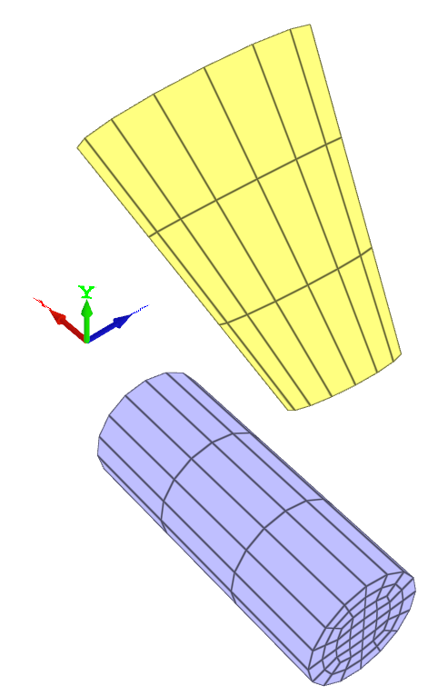
Coordinates for a number of nodes are checked.
Tests
This benchmark is associated with 1 tests.
*COMPONENT_PIPE
Defined in global and local coordinate systems
"Optional title"
coid, pid, N${}_1$, N${}_2$, N${}_3$, csysid, $\alpha_c$
$x_1$, $y_1$, $z_1$, $x_2$, $y_2$, $z_2$, $R_1$, $R_2$
$R_3$, $R_4$
Dimensions and positioning of pipes defined with *COMPONENT_PIPE are verified in this test.
Tested parameters: $pid$, $N_1$, $N_2$, $N_3$, $csysid$, $\alpha_c$, $x_1$, $y_1$, $z_1$, $x_2$, $y_2$, $z_2$, $R_1$, $R_2$, $R_3$ and $R_4$.
Two pipes are created using *COMPONENT_PIPE. One is created in the global coordinate system and the other one in a local coordinate system. Both the origin and the axes in the local coordinate system differs from the global system, as visible in Figure 1.
Parameter $\alpha_c$ is set to 180 deg. for the pipe defined in the global coordinate system. Parameter $R_1$, $R_2$, $R_3$ and $R_4$ are set so that the pipe in the local coordinate system is tapered and hollow.
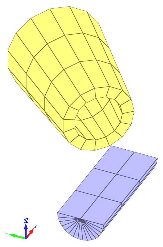
Coordinates for a number of nodes are checked.
Tests
This benchmark is associated with 1 tests.
*COMPONENT_REBAR
Bending
"Optional title"
coid, pid, N${}_x$, N${}_y$, N${}_z$, csysid
$x_1$, $y_1$, $z_1$, $x_2$, $y_2$, $z_2$, $h$
A rebar element with length $L$, diameter $D$ ($L$ >> $D$) and Young's modulus $E$ is fixed at both ends. A transverse displacement, $disp$ ($disp$ < $D$), is defined at the center of the element, causing the element to bend.
The load required to deflect the element to the defined displacement is calculated as:
$$ P = 48EI\cdot \frac{disp}{L^3} $$
$I$ is the second moment of area, defined as:
$$ I = \pi\cdot\frac{D^4}{64} $$
The reaction force in each support should therefore be $P/2$. The reaction forces at termination are checked.
Tests
This benchmark is associated with 1 tests.
Defined in global and local coordinate systems
"Optional title"
coid, pid, N${}_x$, N${}_y$, N${}_z$, csysid
$x_1$, $y_1$, $z_1$, $x_2$, $y_2$, $z_2$, $h$
Dimensions and positioning of rebar grids defined with *COMPONENT_REBAR are verified in this test.
Two rebar grids are created using *COMPONENT_REBAR. One is created in the global coordinate system and the other one in a local coordinate system. Both the origin and the axes in the local coordinate system differs from the global system. The rebar grids consist of one cell in the X-direction, two cells in the Y-direction and three cells in the Z-diretion, as visible in Figure 1.
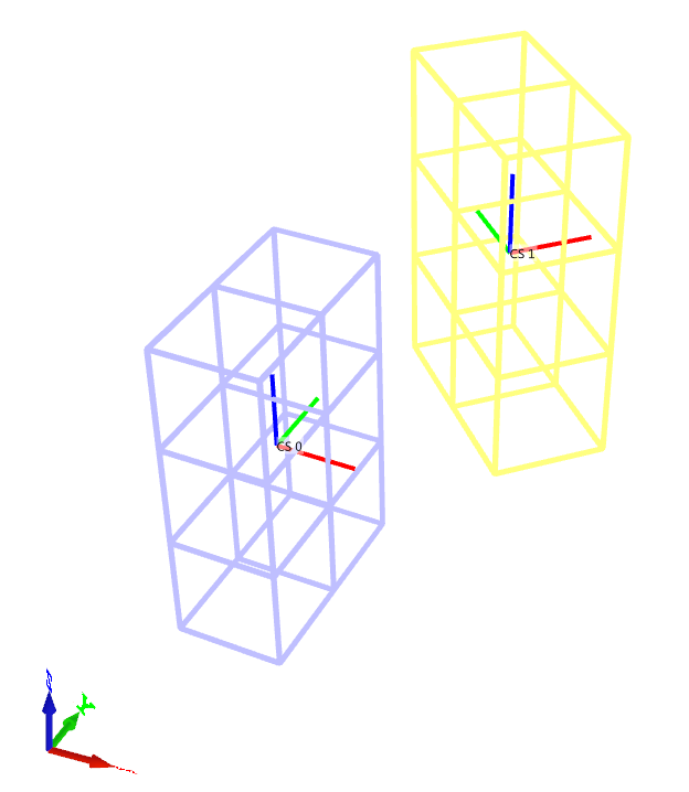
Coordinates for a number of nodes are checked.
Tests
This benchmark is associated with 1 tests.
*COMPONENT_SPHERE
Defined in global and local coordinate systems
"Optional title"
coid, pid, N, N${}_c$, csysid, $\alpha_c$
$x_0$, $y_0$, $z_0$, $R_1$, $R_2$
Dimensions and positioning of spheres defined with *COMPONENT_SPHERE are verified in this test.
Tested parameters: $pid$, $N$, $N_c$, $csysid$, $\alpha_c$, $x_0$, $y_0$, $z_0$, $R_1$, $R_2$.
A sphere and a slice of a sphere are created using *COMPONENT_SPHERE. The sphere is defined in the global coordinate system and the slice in a local coordinate system. Both the origin and the axes in the local coordinate system differs from the global system, as visible in Figure 1. Parameter $\alpha_c$ is set to 180°. in the slice.
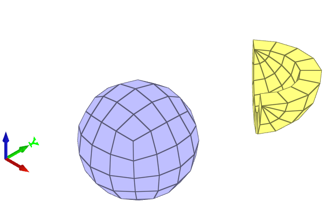
Coordinates for a number of nodes are checked.
Tests
This benchmark is associated with 1 tests.
*CONNECTOR_DAMPER
Axially loaded damper
"Optional title"
coid
pid${}_1$, pid${}_2$, csysid, $R$, $h$, $m$, $\eta$, $k_{max}$
cid${}_{axial}$, cid${}_{shear}$, cid${}_{bend}$, cid${}_{rate}$
Tested parameters: coid, pid1, pid2, csysid, R, h, m, η, kmax, cidaxial, cidshear, cidbend, cidrate.
This model tests the command *CONNECTOR_DAMPER. It consists of two tests, one with quasi-static and one with a dynamic response.
An axially loaded damper is positioned between two plates with the command *CONNECTOR_DAMPER. It is first compressed and then loaded in tension. The base plate is restricted in all directions while the top plate is assigned a motion in the negative and positive Z-direction.
See Figure 1.
The damper properties are the same for both tests but the prescribed velocity of the top plate differs.
-Velocity (Quasi-static) = $0.01 \ m/s$
-Velocity (Dynamic) = $1 \ m/s$
The quasi-static as well as the dynamic response of the dampers can be seen in Figure 2.
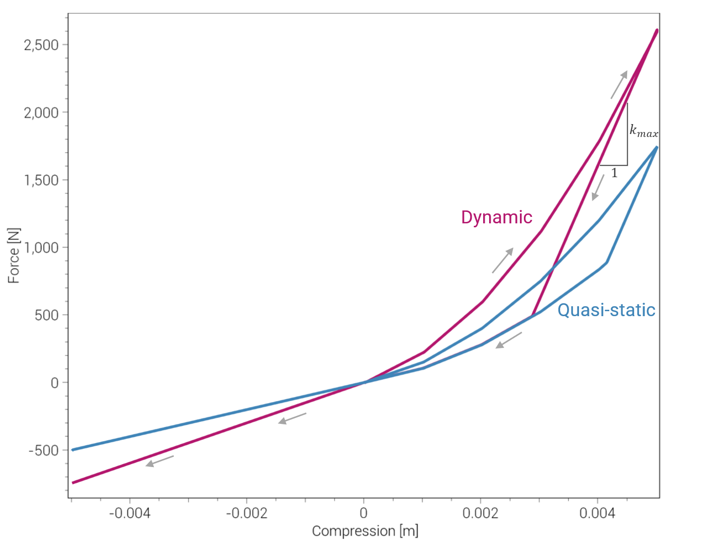
Maximum and minimum normal force and displacement in Z direction is checked for version control.
Tests
This benchmark is associated with 2 tests.
*CONNECTOR_GLUE_LINE
Combined stress
"Optional title"
coid
entype${}_1$, enid${}_1$, entype${}_2$, enid${}_2$, pathid, $tol$, $\Delta$, $w$
$h$, $\rho$, $E$, $\nu$, $\sigma_f$, $\tau_f$, $G_I$, $G_{II}$
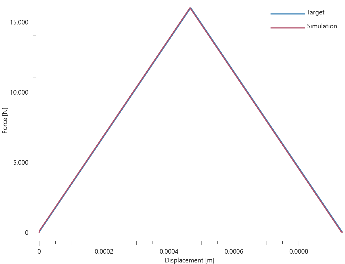
This test is similair to the test "*CONNECTOR_GLUE_LINE - Normal stress". In the current test, the glue is subjected to a combination of normal and shear stress instead.
Tested parameters: $w$, $h$, $E$, $\nu$, $\sigma_f$, $\tau_f$, $G_I$ and $G_{II}$.
Forces vs. displacements are presented in Figure 1 and 2 together with target curves of the analytical solutions.
Maximum and average value of the forces, delamination energy and area are checked.
Tests
This benchmark is associated with 1 tests.
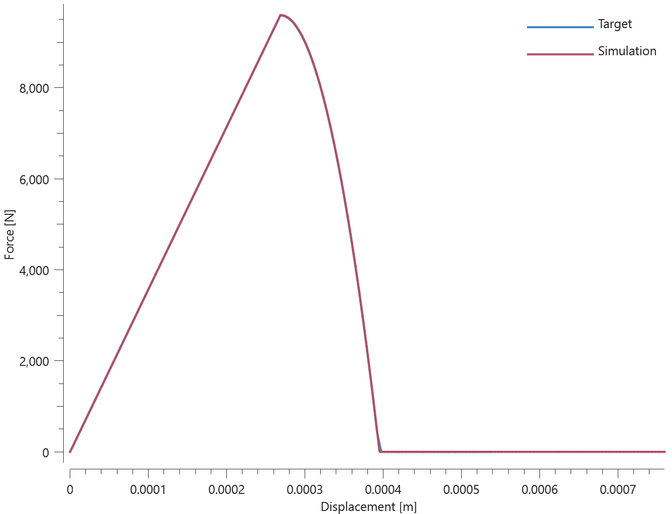
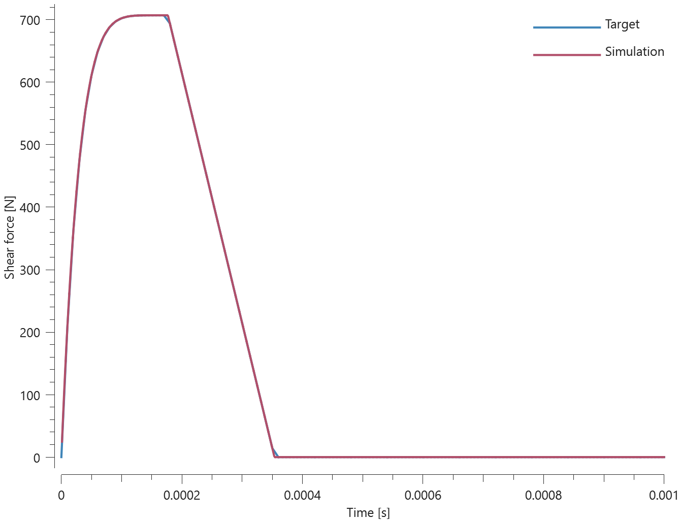
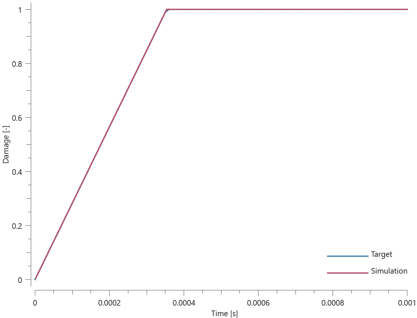
Normal stress
"Optional title"
coid
entype${}_1$, enid${}_1$, entype${}_2$, enid${}_2$, pathid, $tol$, $\Delta$, $w$
$h$, $\rho$, $E$, $\nu$, $\sigma_f$, $\tau_f$, $G_I$, $G_{II}$
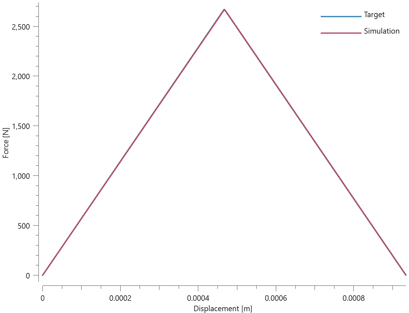
The glue properties of *CONNECTOR_GLUE_LINE in a state of normal stress is verified in this test.
Tested parameters: $w$, $h$, $E$, $\nu$, $\sigma_f$ and $G_I$.
Two quadratic plates with length 100 mm and thickness 10 mm are glued together with *CONNECTOR_GLUE_LINE. The glue line has a width of 5 mm and a thickness of 1 mm. The glue line runs 10 mm from the edges around the plate, as illustrated in Figure 1.
Prescribed motions causing a state of normal stress in the glue are imposed on the plates. Force vs. displacement from the simulation is presented in Figure 2 together with a target curve of the analytical solution.
Maximum and average value of the force, delamination energy and area are checked.
Tests
This benchmark is associated with 1 tests.
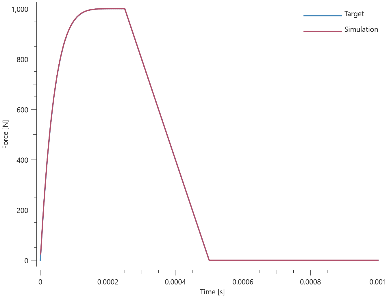
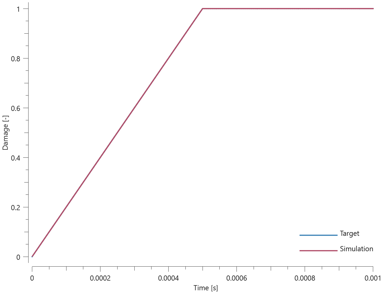
Shear stress
"Optional title"
coid
entype${}_1$, enid${}_1$, entype${}_2$, enid${}_2$, pathid, $tol$, $\Delta$, $w$
$h$, $\rho$, $E$, $\nu$, $\sigma_f$, $\tau_f$, $G_I$, $G_{II}$
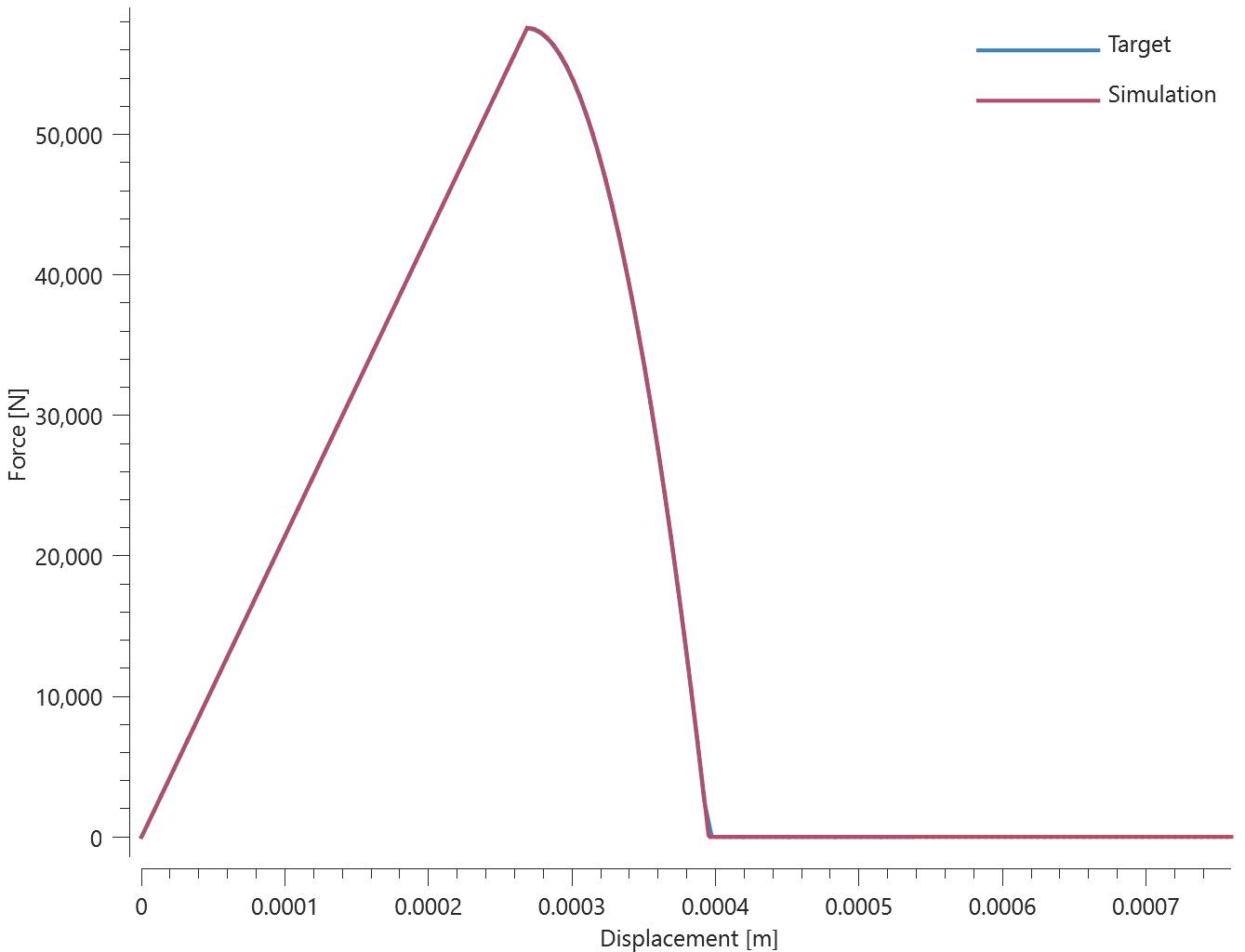
This test is similair to the test "*CONNECTOR_GLUE_LINE - Normal stress". In the current test, the glue is subjected to a state of shear stress instead.
Tested parameters: $w$, $h$, $E$, $\nu$, $\tau_f$ and $G_{II}$.
Force vs. displacement from the simulation is presented in Figure 1 together with a target curve of the analytical solution.
Maximum and average value of the force, delamination energy and area are checked.
Tests
This benchmark is associated with 1 tests.
*CONNECTOR_GLUE_SURFACE
Combined stress
"Optional title"
coid
entype${}_1$, enid${}_1$, entype${}_2$, enid${}_2$, $tol$
$h$, $\rho$, $E$, $\nu$, $\sigma_f$, $\tau_f$, $G_I$, $G_{II}$
This test is similair to the test "*CONNECTOR_GLUE_SURFACE - Normal stress". In the current test, the glue is subjected to a combination of normal and shear stress instead.
Tested parameters: $h$, $E$, $\nu$, $\sigma_f$, $\tau_f$, $G_I$ and $G_{II}$.
Forces vs. displacements are presented in Figure 1 and 2 together with target curves of the analytical solutions.
Maximum and average value of the forces, delamination energy and area are checked.
Tests
This benchmark is associated with 1 tests.
Normal stress
"Optional title"
coid
entype${}_1$, enid${}_1$, entype${}_2$, enid${}_2$, $tol$
$h$, $\rho$, $E$, $\nu$, $\sigma_f$, $\tau_f$, $G_I$, $G_{II}$
The glue properties of *CONNECTOR_GLUE_SURFACE in a state of normal stress is verified in this test.
Tested parameters: $h$, $E$, $\nu$, $\sigma_f$ and $G_I$.
Two quadratic plates with length 100 mm and thickness 10 mm are glued together with *CONNECTOR_GLUE_SURFACE. Prescribed motions causing a state of normal stress in the glue are imposed on the plates.
Force vs. displacement from the simulation is presented in Figure 1 together with a target curve of the analytical solution.
Maximum and average value of the force, delamination energy and area are checked.
Tests
This benchmark is associated with 1 tests.
Shear stress
"Optional title"
coid
entype${}_1$, enid${}_1$, entype${}_2$, enid${}_2$, $tol$
$h$, $\rho$, $E$, $\nu$, $\sigma_f$, $\tau_f$, $G_I$, $G_{II}$
This test is similair to the test "*CONNECTOR_GLUE_SURFACE - Normal stress". In the current test, the glue is subjected to a state of shear stress instead.
Tested parameters: $h$, $E$, $\nu$, $\tau_f$ and $G_{II}$.
Force vs. displacement from the simulation is presented in Figure 1 together with a target curve of the analytical solution.
Maximum and average value of the force, delamination energy and area are checked.
Tests
This benchmark is associated with 1 tests.
*CONNECTOR_RIGID
Connection in motion
"Optional title"
coid, entype, enid
*CONNECTOR_RIGID is verified in this test.
Tested parameters: $entype$ and $enid$.
Two rigid elements are connected with a rigid connection. One of the elements is set in motion. The displacement and velocity in the other element is checked at termination.
Tests
This benchmark is associated with 1 tests.
*CONNECTOR_SPOT_WELD
Combined stress
"Optional title"
coid
entype, enid, tid, $tol$
$R$, $h$, $m$, $k$, $F_t$, $F_s$, $W_t$, $W_s$
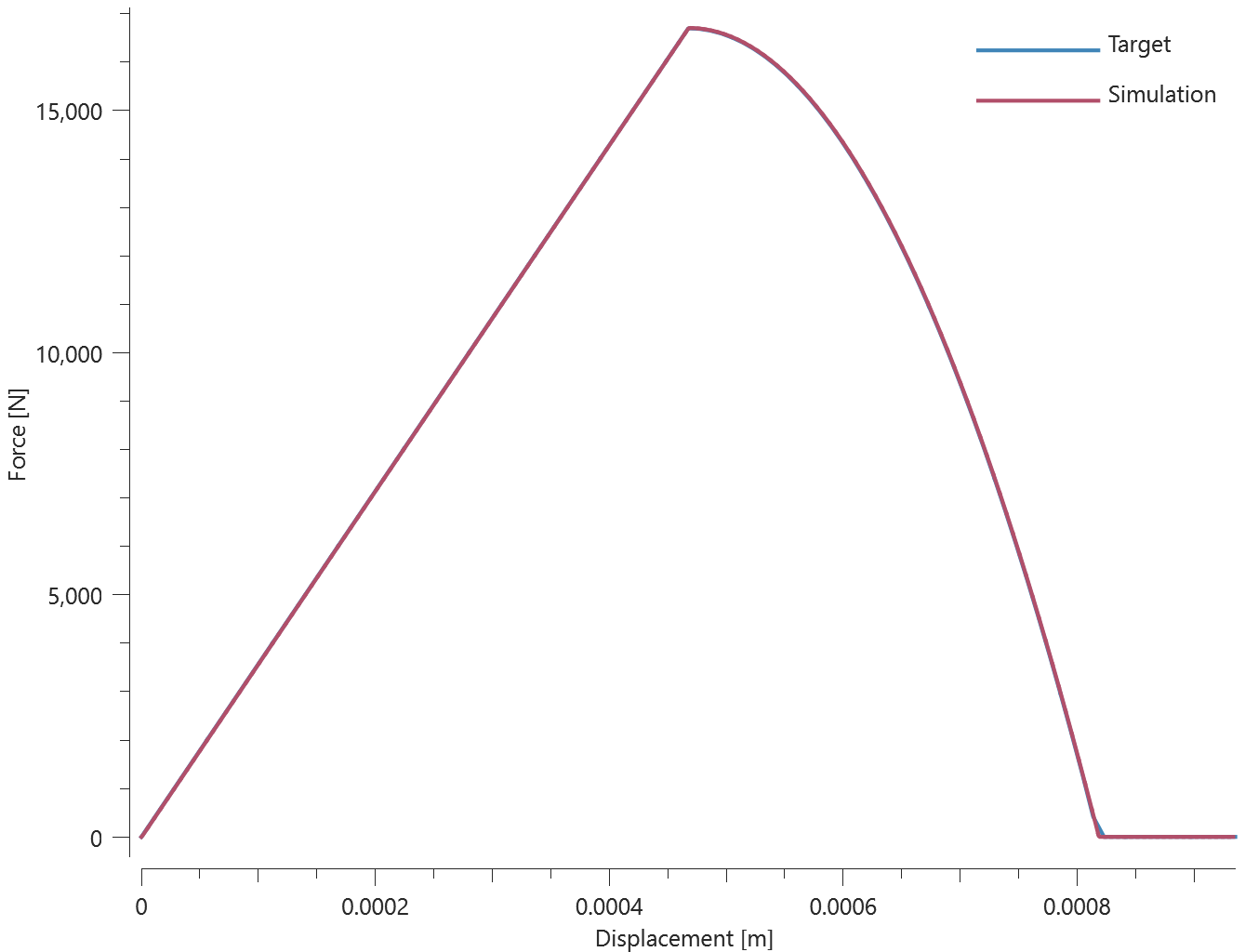
This test is similair to the test "*CONNECTOR_SPOT_WELD - Normal stress". In the current test, the spot welds are subjected to a combination of normal and shear stress instead.
Tested parameters: $R$, $h$, $k$, $F_t$, $F_s$, $W_t$ and $W_s$.
The resultant force vs. displacement from the simulation is presented in Figure 1 together with a target curve of the analytical solution.
Maximum and average value of the force and dissipated energy are checked.
Tests
This benchmark is associated with 1 tests.
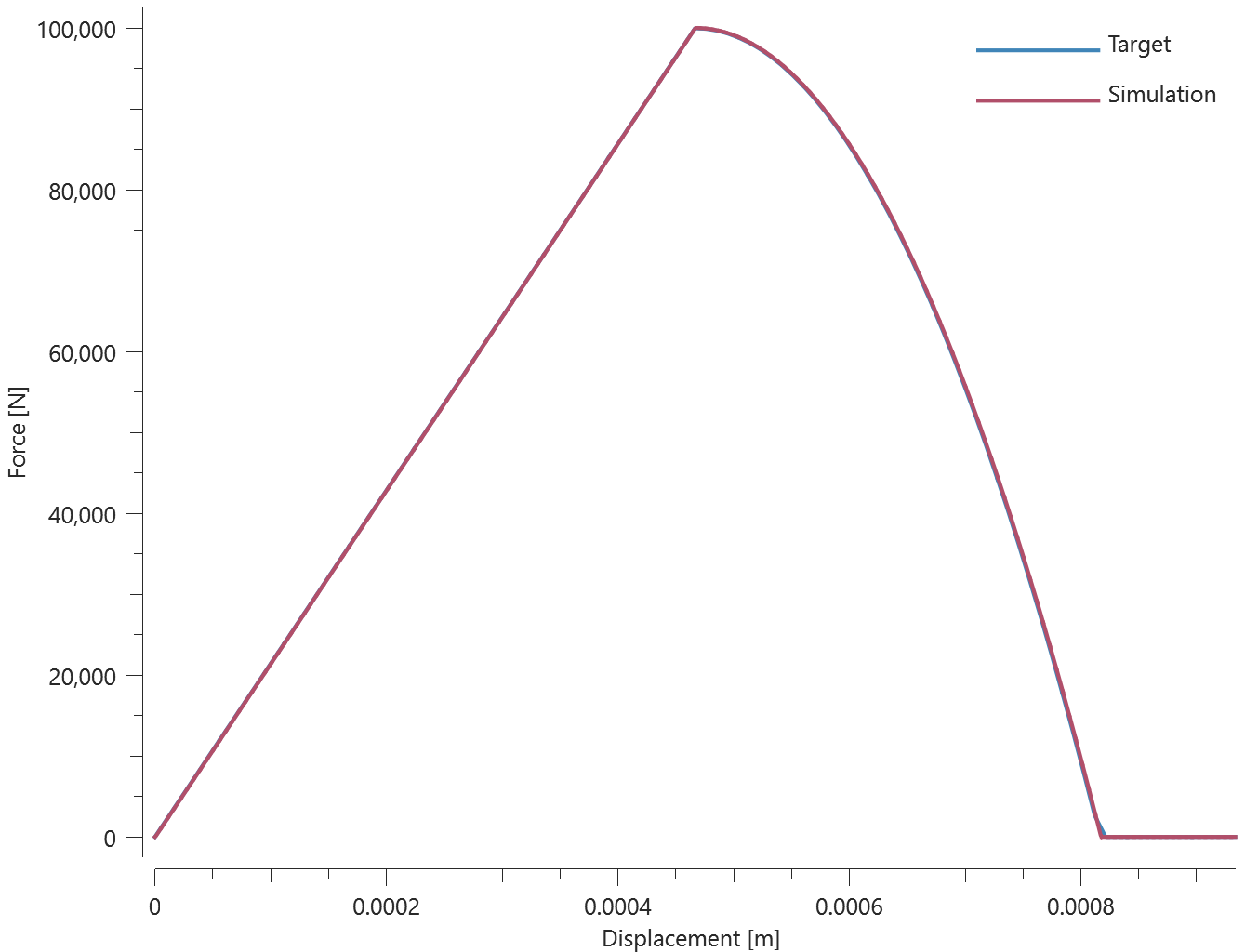
Normal stress
"Optional title"
coid
entype, enid, tid, $tol$
$R$, $h$, $m$, $k$, $F_t$, $F_s$, $W_t$, $W_s$
The spot weld properties of *CONNECTOR_SPOT_WELD in a state of normal stress is verified in this test.
Tested parameters: $R$, $h$, $k$, $F_t$ and $W_t$.
Two quadratic plates with length 200 mm and thickness 10 mm are connected to each other by four spot welds defined with *CONNECTOR_SPOT_WELD as illustrated in Figure 1.
Prescribed motions causing a state of normal stress in the spot welds are imposed on the plates. Force vs. displacement from the simulation is presented in Figure 2 together with a target curve of the analytical solution.
Maximum and average value of the force and dissipated energy are checked.
Tests
This benchmark is associated with 1 tests.
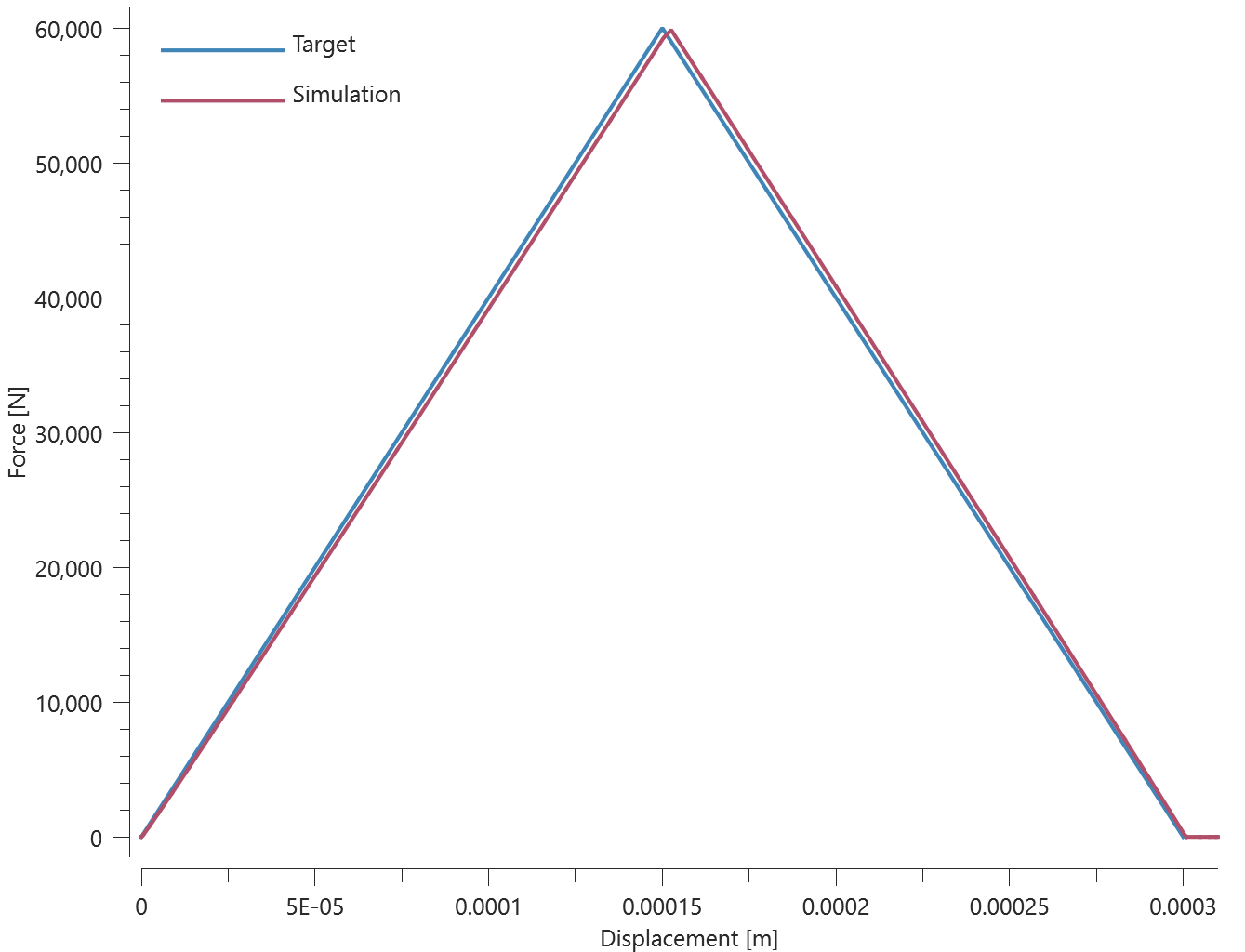
Shear stress
"Optional title"
coid
entype, enid, tid, $tol$
$R$, $h$, $m$, $k$, $F_t$, $F_s$, $W_t$, $W_s$
This test is similair to the test "*CONNECTOR_SPOT_WELD - Normal stress". In the current test, the spot welds are subjected to a state of shear stress instead.
Tested parameters: $R$, $h$, $k$, $F_s$ and $W_s$.
Force vs. displacement from the simulation is presented in Figure 1 together with a target curve of the analytical solution.
Maximum and average value of the force and dissipated energy are checked.
Tests
This benchmark is associated with 1 tests.
*CONNECTOR_SPOT_WELD_NODE
Normal stress
"Optional title"
coid, nid, pid, N, entype, enid
This test is equivalent to the test "*CONNECTOR_SPOT_WELD - Normal stress". The only difference is the input format, in which *CONNECTOR_SPOT_WELD_NODE is used to define the connector location of the spot welds from Node ID. The command is used in combination with *PROP_SPOT_WELD.
All parameters used are the same as in the test "*CONNECTOR_SPOT_WELD - Normal stress", which means that the same result is expected.
Tests
This benchmark is associated with 1 tests.
*CONNECTOR_SPR
Combined stress
"Optional title"
coid, pid${}_s$, pid${}_m$, csysid
$R$, $h$, $m$, $f_n^{max}$, $f_t^{max}$, $d_n^{max}$, $d_t^{max}$, $\xi_n$
$\xi_t$, $a_1$, $a_2$, $a_3$
This test is similair to the test "*CONNECTOR_SPR - Normal stress". In the current test, the rivet is subjected to a combination of normal and shear stress instead.
Tested parameters: $R$, $h$, $f_n^{max}$, $f_t^{max}$, $d_n^{max}$, $d_t^{max}$, $\xi_n$, $\xi_t$, $a_1$, $a_2$ and $a_3$.
Forces vs. time and damage vs. time from the simulation are presented in Figure 1, 2 and 3 together with target curves from a verification script.
Maximum and average forces and damage in the rivet are checked in spr.out. The dissipated energy is also checked for version control.
Tests
This benchmark is associated with 1 tests.
Normal stress
"Optional title"
coid, pid${}_s$, pid${}_m$, csysid
$R$, $h$, $m$, $f_n^{max}$, $f_t^{max}$, $d_n^{max}$, $d_t^{max}$, $\xi_n$
$\xi_t$, $a_1$, $a_2$, $a_3$
The rivet properties of *CONNECTOR_SPR in a state of normal stress is verified in this test.
Tested parameters: $R$, $h$, $f_n^{max}$, $d_n^{max}$, $\xi_n$, $a_1$, $a_2$ and $a_3$.
Two plates are connected to each other by a self-piercing rivet. Prescribed motions causing a state of normal stress in the rivet are imposed on the plates. Force vs. time and damage vs. time from the simulation are presented in Figure 1 and 2 together with target curves from a verification script.
Maximum and average force and damage in the rivet are checked in spr.out. The dissipated energy is also checked for version control.
Tests
This benchmark is associated with 1 tests.
Shear stress
"Optional title"
coid, pid${}_s$, pid${}_m$, csysid
$R$, $h$, $m$, $f_n^{max}$, $f_t^{max}$, $d_n^{max}$, $d_t^{max}$, $\xi_n$
$\xi_t$, $a_1$, $a_2$, $a_3$
This test is similair to the test "*CONNECTOR_SPR - Normal stress". In the current test, the rivet is subjected to a state of shear stress instead.
Tested parameters: $R$, $h$, $f_t^{max}$, $d_t^{max}$, $\xi_t$, $a_1$, $a_2$ and $a_3$.
Force vs. time and damage vs. time from the simulation are presented in Figure 1 and 2 together with target curves from a verification script.


Maximum and average force and damage in the rivet are checked in spr.out. The dissipated energy is also checked for version control.
Tests
This benchmark is associated with 1 tests.
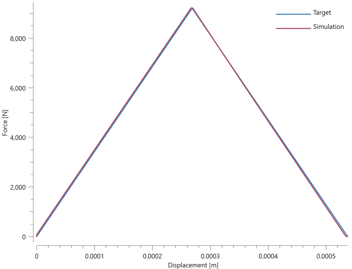
*CONNECTOR_SPRING
Intrinsic operations (dnorm, dnorm_min, dnorm_max)
coid, N${}_1$, N${}_2$, $m$, $k$, $\xi$, $F_{fail}$, direc, $l_0$
Intrinsic operations (dnorm, dnorm_min, dnorm_max) are verified in this test.
Tested parameters: coid, N1, N2, m, k
The model contains three springs with different functions defining elastic force versus elongation. The springs are clamped at one end and are given a prescribed displacement at the other end.
The springs have the following properties:
Spring 1:
$$ F_1(t) = dnorm $$
Spring 2:
$$ F_2(t) = dnorm\_min $$
Spring 3:
$$ F_3(t) = dnorm\_max $$
The prescribed displacement of the free nodes is presented in Table 1.
| Time | X-coordinate |
|---|---|
| 0.0 | 0.0 |
| 0.2 | 0.1 |
| 0.4 | -0.1 |
| 0.6 | 0.2 |
| 0.8 | 0.1 |
| 1.0 | 0.0 |
Force vs. time for the springs is presented in Figure 1.
/connector_spring_intrinsic_operations.png)
The spring forces are checked at termination.
Tests
This benchmark is associated with 1 tests.
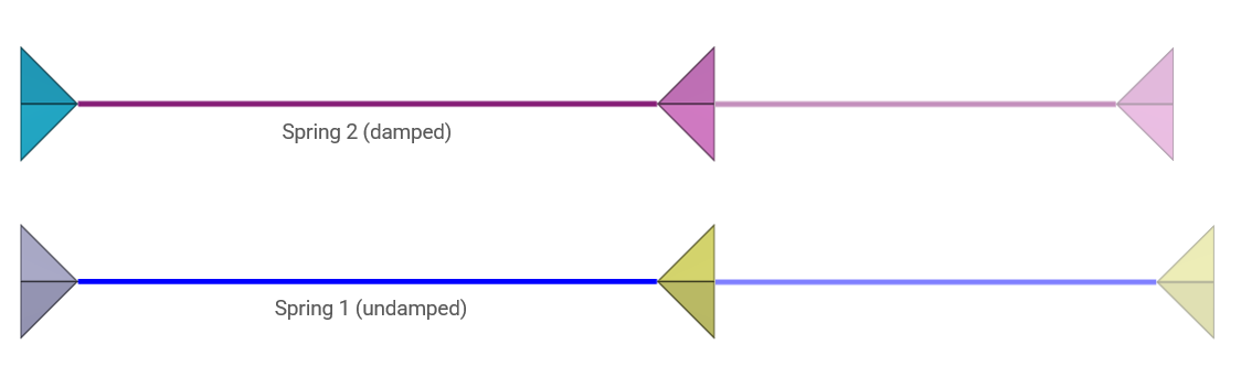
Linear springs
coid, N${}_1$, N${}_2$, $m$, $k$, $\xi$, $F_{fail}$, direc, $l_0$
Linear stiffness and damping in *CONNECTOR_SPRING are verified in this test.
Tested parameters: $N_1$, $N_2$, $m$, $k$ and $\xi$.
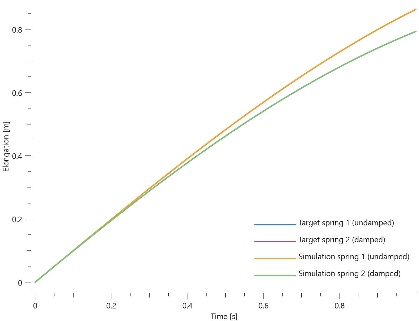
The model contains two springs with constant stiffness $k$ and mass $m$. The node mass is $m/2$. The springs are clamped at one end and are given an initial velocity $v_0$ at the other end. Spring 1 is undamped and spring 2 is damped. The absolute damping $c$ is defined as a fraction $\xi$ of the critical damping of the springs highest eigenfrequency $\omega_{max}$.
Analytical displacement, spring 1 (undamped):
$$ \omega_0 = \sqrt{\frac{2k}{m}} %= 4.47214 rad/s $$
$$ x_1 (t) = \frac{v_0}{\omega_0}\cdot sin (\omega_0 t) $$
Displacement at time $t = 1$, spring 1:
$$ x_1 (1) = \frac{v_0}{\omega_0}\cdot sin (\omega_0) %= -0.21718 $$
Analytical displacement, spring 2 (damped):
$$ \xi_2 = \frac{c}{\sqrt{2mk}} = \sqrt{2}\cdot \xi %= 0.14142 $$
$$ \omega_d = \omega_0\cdot \sqrt{1-{\xi_2}^2} %= 4.42719 rad/s $$
$$ x_2 (t) = \frac{v_0}{\omega_d}\cdot sin(\omega_d t)\cdot exp(-\xi_2\cdot \omega_0 t) $$
Displacement at time $t = 1$, spring 2:
$$ x_2 (1) = \frac{v_0}{\omega_d}\cdot sin(\omega_d)\cdot exp(-\xi_2\cdot \omega_0) %= -0.11516 $$
The spring displacements are checked at termination.
Tests
This benchmark is associated with 1 tests.
Nonlinear springs
coid, N${}_1$, N${}_2$, $m$, $k$, $\xi$, $F_{fail}$, direc, $l_0$
Non-linear stiffness and damping in *CONNECTOR_SPRING are verified in this test.
Tested parameters: $N_1$, $N_2$, $m$, $k$ and $\xi$.
The model contains two springs with non-linear force-displacement and damping properties. The springs are clamped at one end and given a prescribed velocity $v=1$ at the other end. Velocity and displacement at a given moment $t$ takes trivial values.
$$ v_{norm} = v = 1 $$
$$ d_{norm} = \int v_{norm}dt = v_{norm}t = t $$
The force at $t = 1$, spring 1:
$$ F_1(1) = \exp(d_{norm}) = \exp(t) = e %\approx 2.718 $$
The force at $t = 1$, spring 2:
$$ F_2(1) = d_{norm} + \exp(v_{norm}) = t + \exp(t) = 1 + e %\approx 3.718 $$
The spring forces are checked at termination.
Tests
This benchmark is associated with 1 tests.
State file output
coid, N${}_1$, N${}_2$, $m$, $k$, $\xi$, $F_{fail}$, direc, $l_0$
This model tests the unloaded spring length, parameter $l_{0}$ in *CONNECTOR_SPRING , which is used when importing results in subsequent simulations. The test consists of 2 steps. The *CONNECTOR_SPRING command with parameter $l_{0}$ is automatically generated by the solver engine in the state file impetus_state_spring1.k at termination.
The model contains two springs with constant stiffness $k$ and mass $m$. The node mass is $m/2$. The springs are clamped at one end and are given an initial velocity $v_0$ at the other end. Spring 1 is undamped and spring 2 is damped. The absolute damping $c$ is defined as a fraction $\xi$ of the critical damping of the springs highest eigenfrequency $\omega_{max}$.
Analytical displacement, spring 1 (undamped):
$$ \omega_0 = \sqrt{\frac{2k}{m}} $$
$$ x_1 (t) = \frac{v_0}{\omega_0}\cdot sin (\omega_0 t) $$
Displacement at time $t = 1$, spring 1:
$$ x_1 (1) = \frac{v_0}{\omega_0}\cdot sin (\omega_0) $$
Analytical displacement, spring 2 (damped):
$$ \xi_2 = \frac{c}{\sqrt{2mk}} = \sqrt{2}\cdot \xi $$
$$ \omega_d = \omega_0\cdot \sqrt{1-{\xi_2}^2} $$
$$ x_2 (t) = \frac{v_0}{\omega_d}\cdot sin(\omega_d t)\cdot exp(-\xi_2\cdot \omega_0 t) $$
Displacement at time $t = 1$, spring 2:
$$ x_2 (1) = \frac{v_0}{\omega_d}\cdot sin(\omega_d)\cdot exp(-\xi_2\cdot \omega_0) $$
The test setup can be seen in Figure 1.
Spring elongation vs. time for step 1 can be seen in Figure 2 together with a target curve from a verification script.
Spring elongation vs. time for step 2 can be seen in Figure 3 together with a target curve from a verification script.
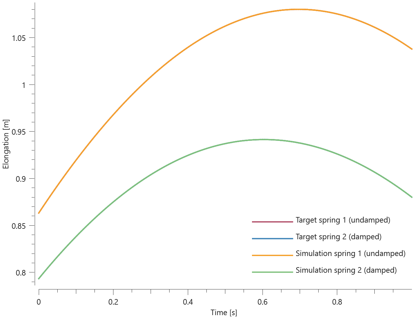
The spring displacements are checked for version control.
Tests
This benchmark is associated with 2 tests.
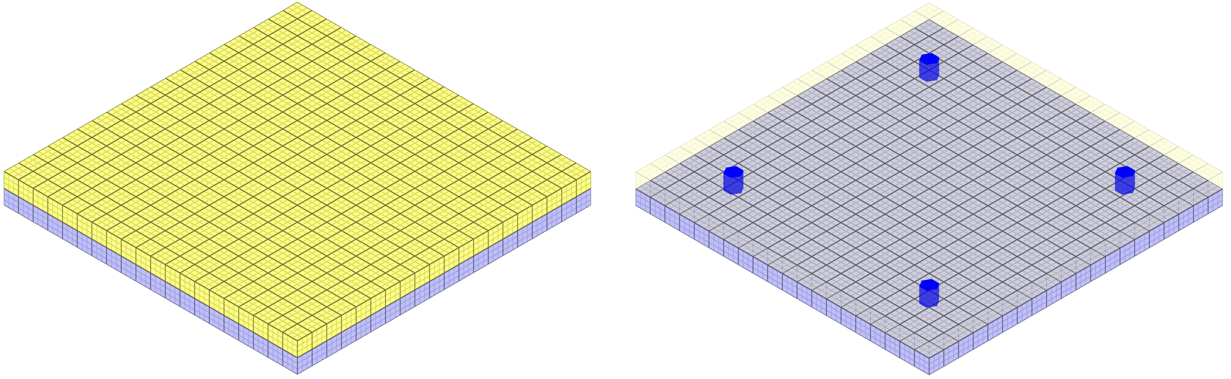
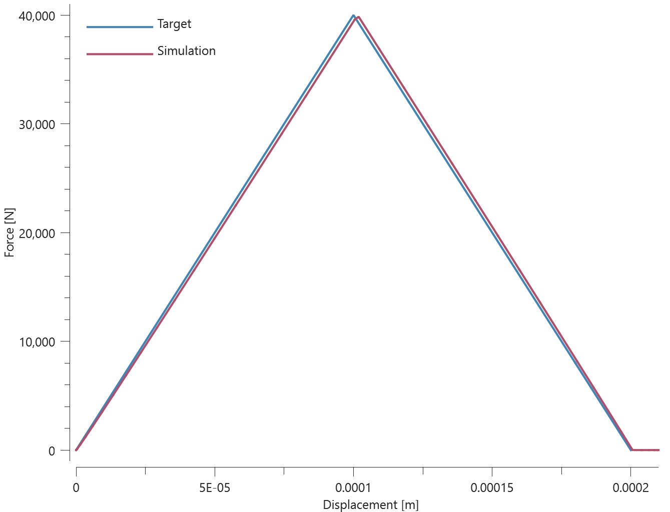
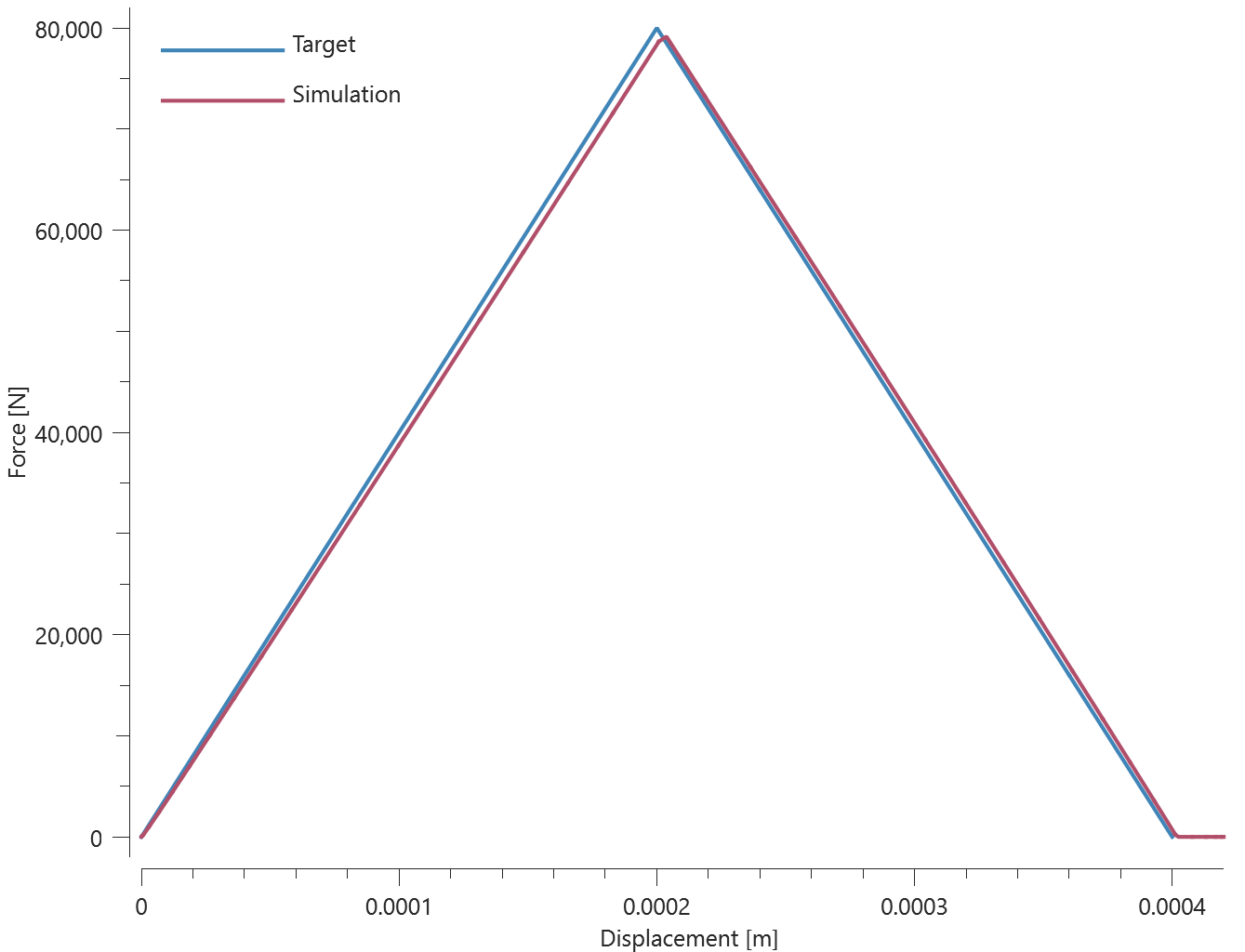
*CONTACT
Contact and friction forces between all element types
"Optional title"
coid, accuracy_level, accuracy_edge
entype${}_1$, enid${}_1$, entype${}_2$, enid${}_2$, $\mu$, $pfac$, $t_{beg}$, $t_{end}$
merge, $\xi$, gid${}_0$, gid${}_1$, $\delta_{0}^{offset}$, $\delta_{0}^{max}$, $\delta^{edge}$
fid${}_{wear1}$, fid${}_{wear2}$, fid${}_{thermal}$, $\alpha_{edge}$, one_way, no_internal, $\sigma_{stick}$, fric_heat
Contact and friction forces between all element types are verified in this test.
Tested parameters: $pfac$ (automatic calculation of penalty stiffness) and $\mu$.
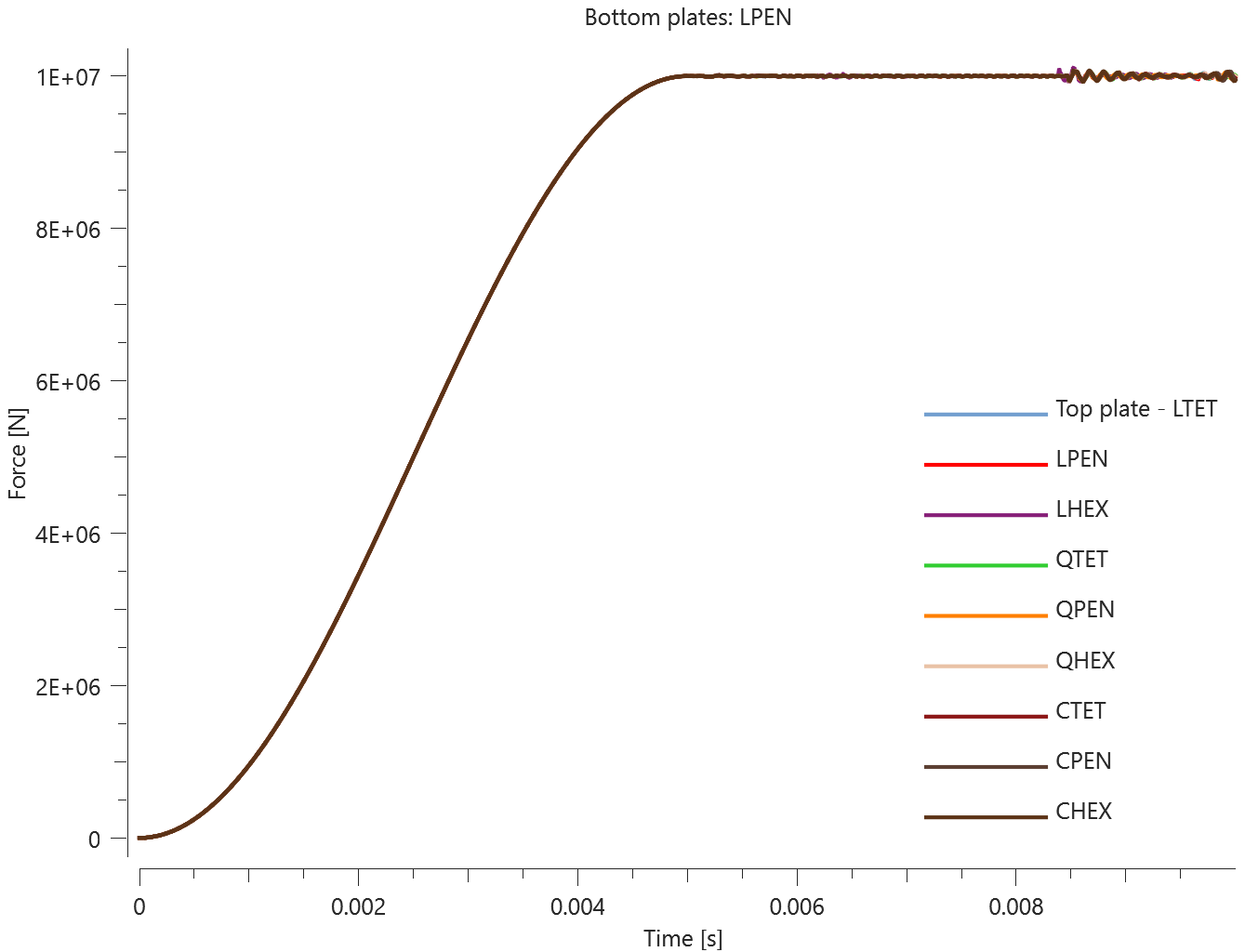
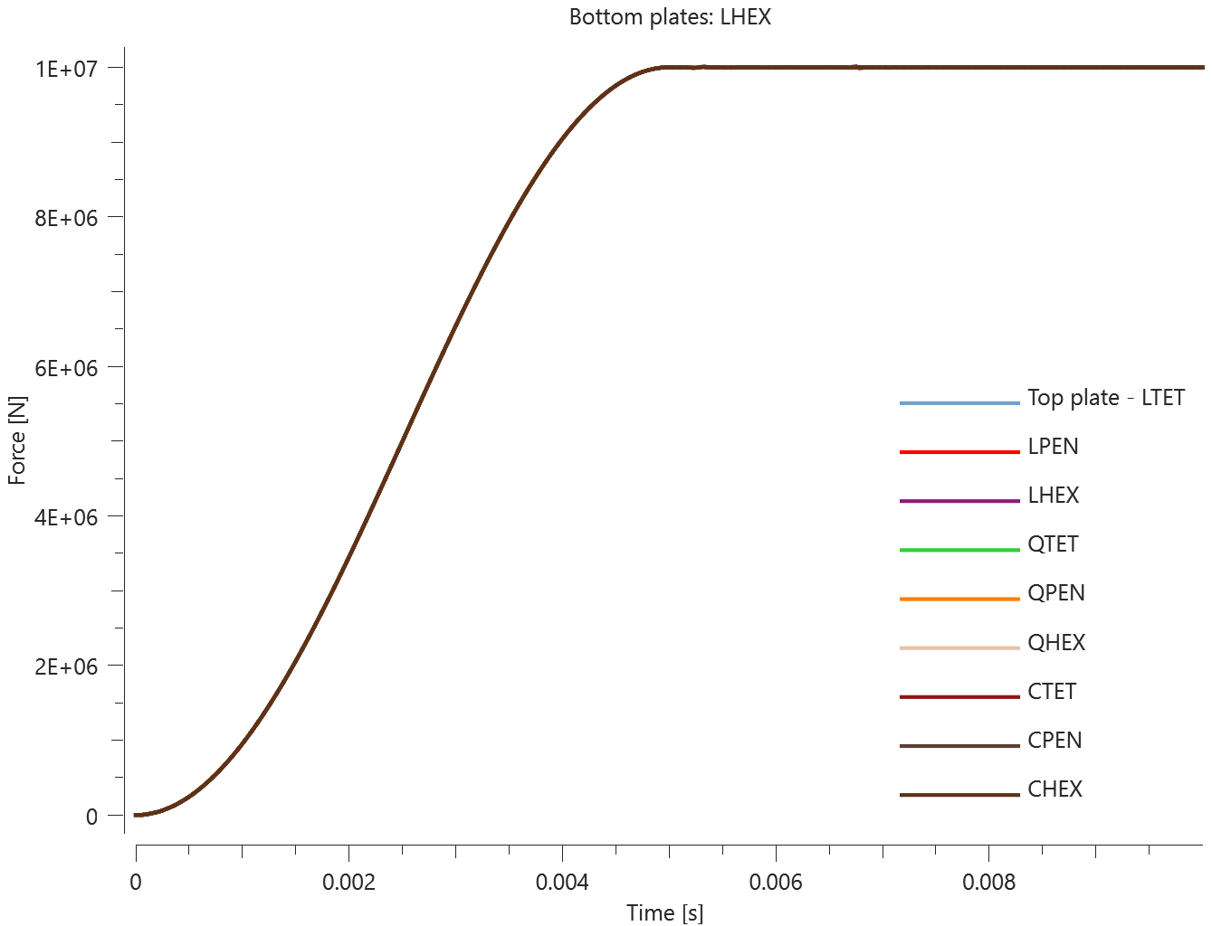
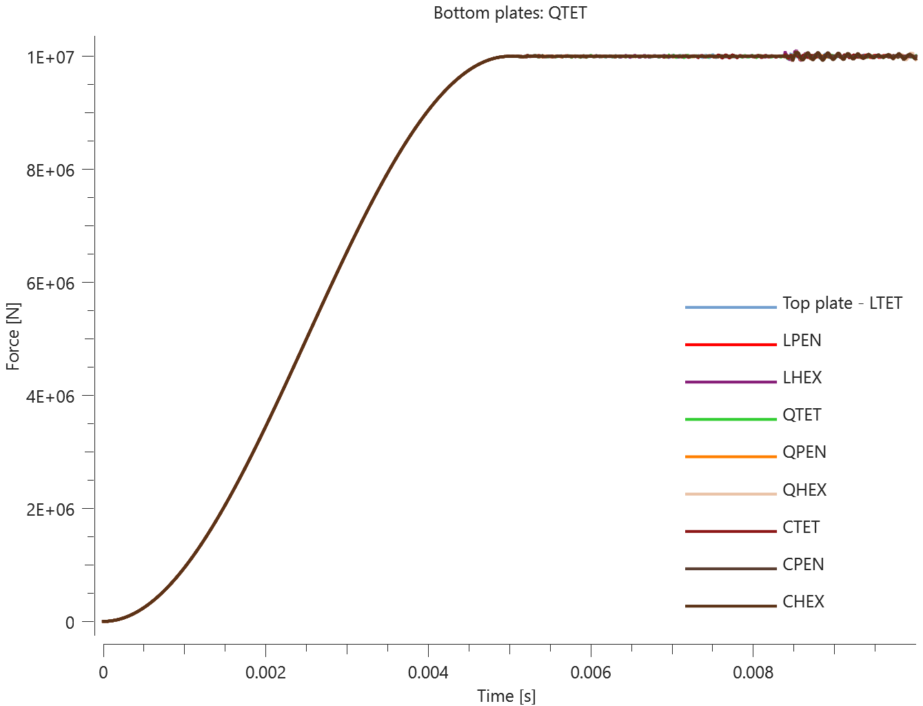
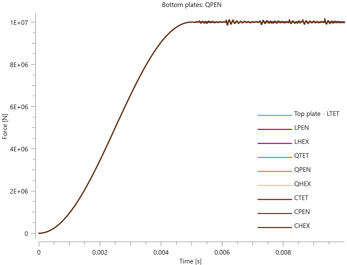
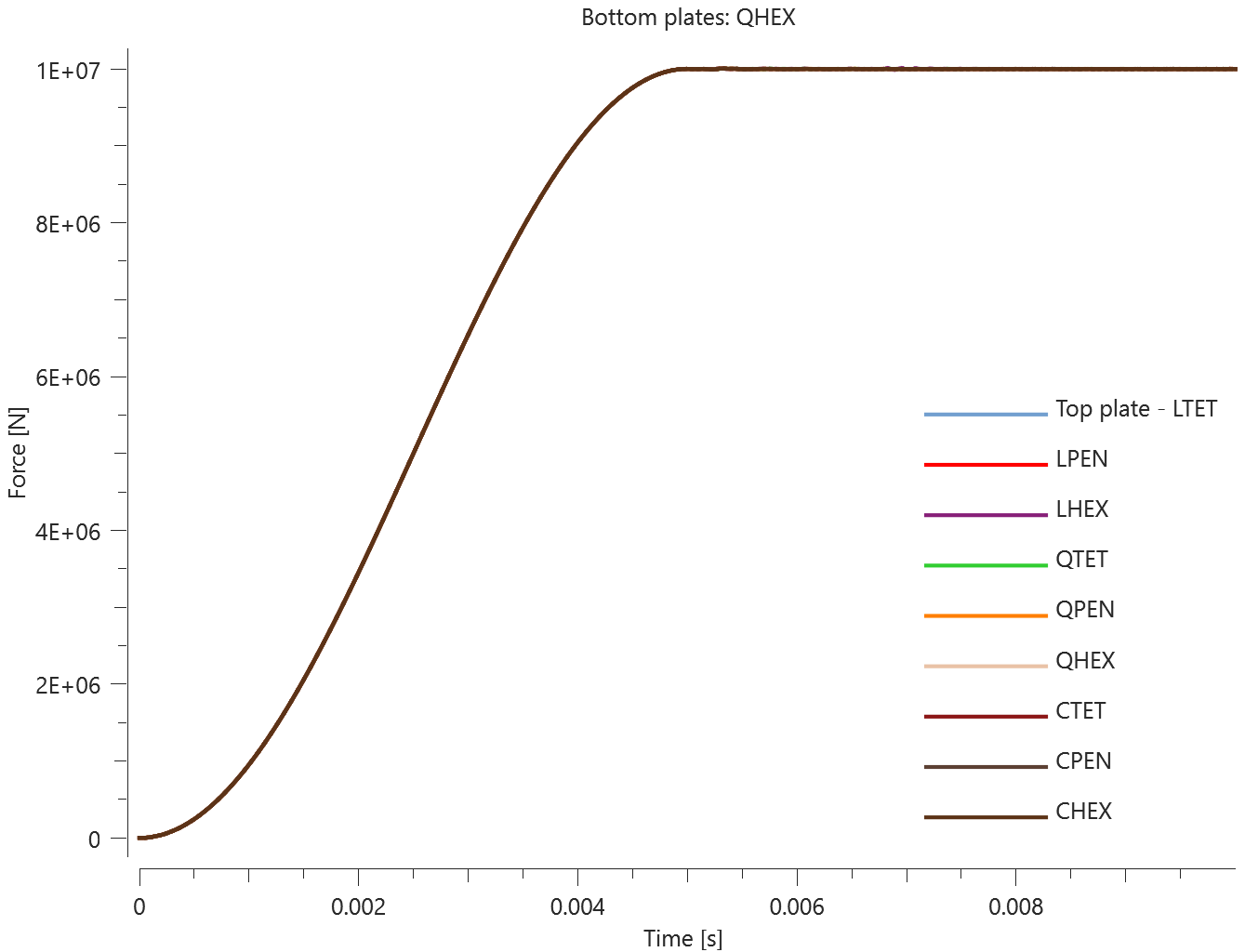
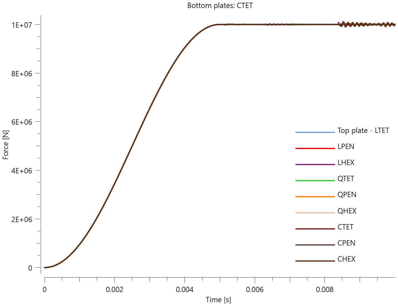
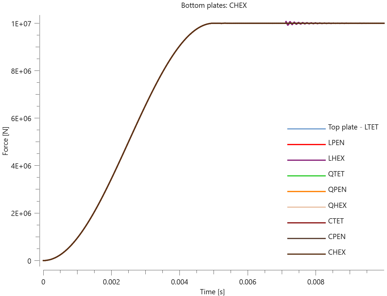
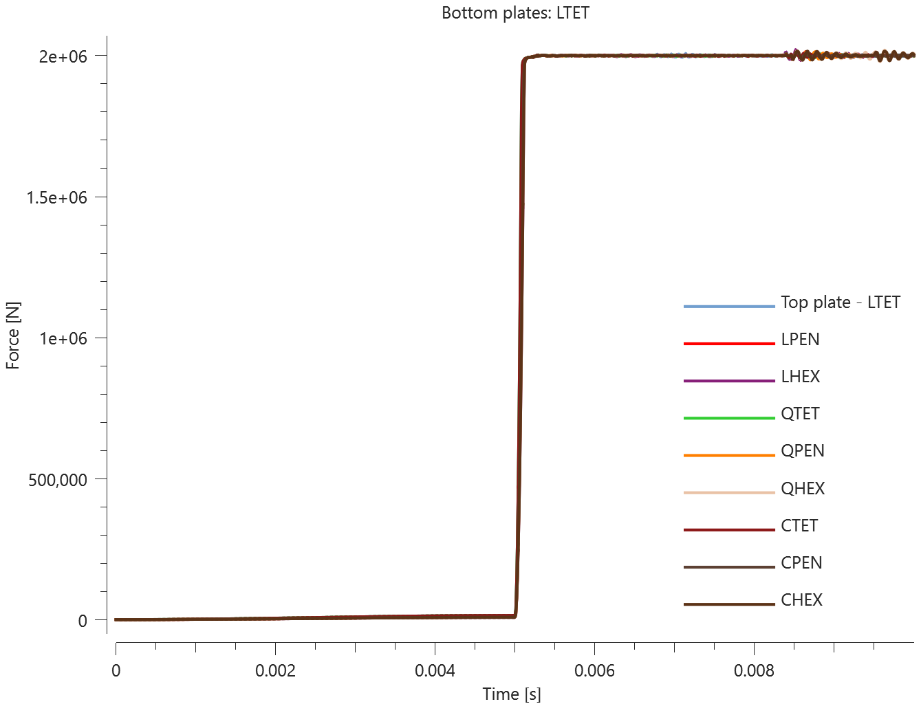
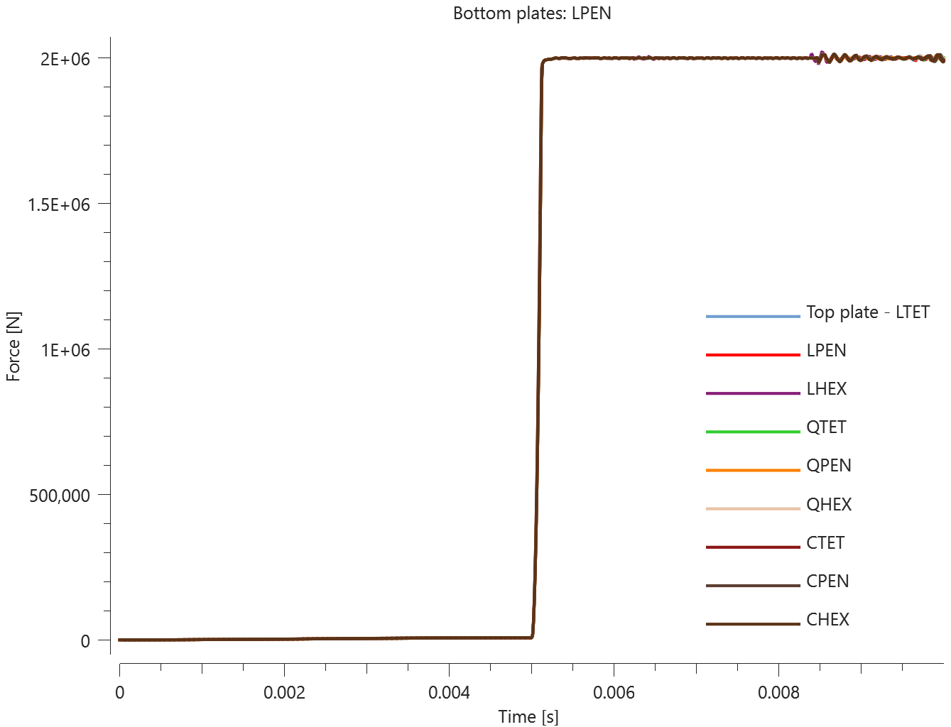
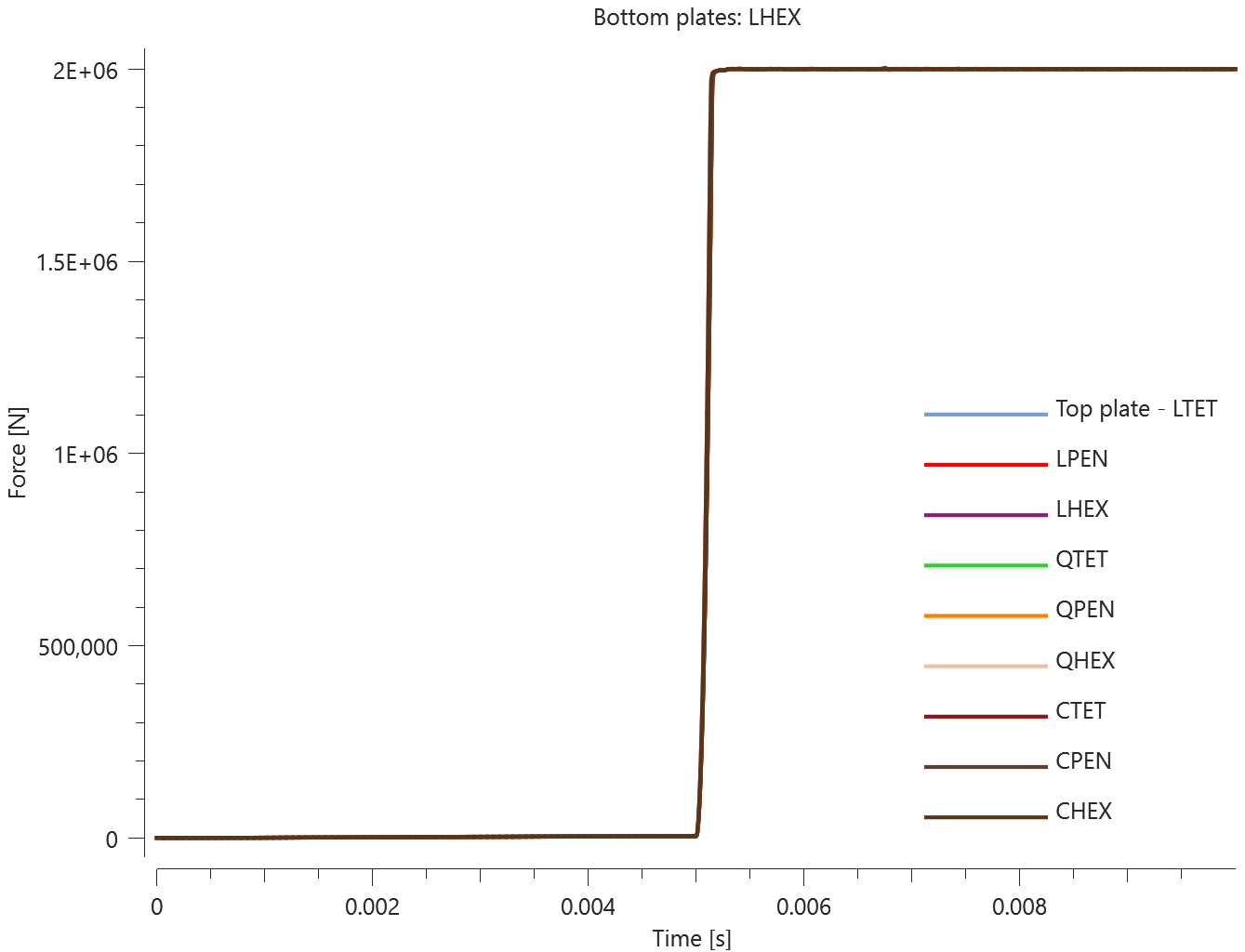
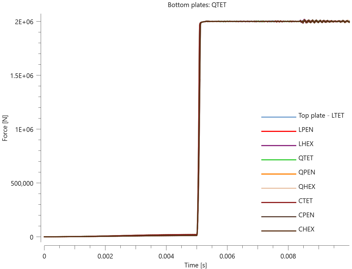
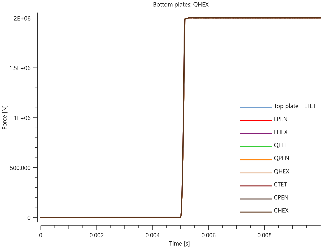
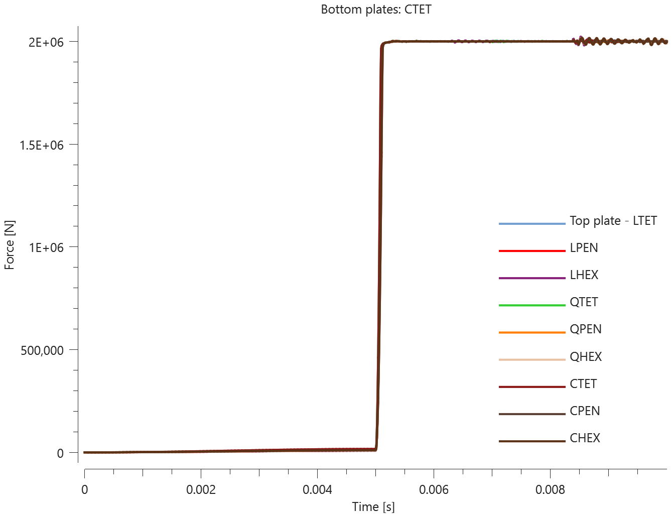
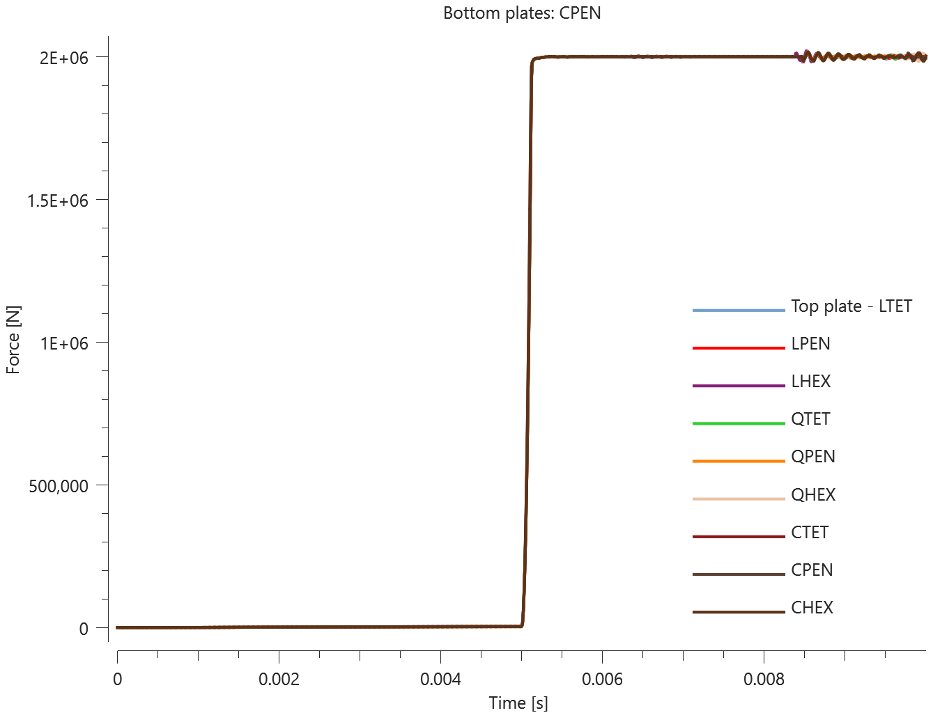
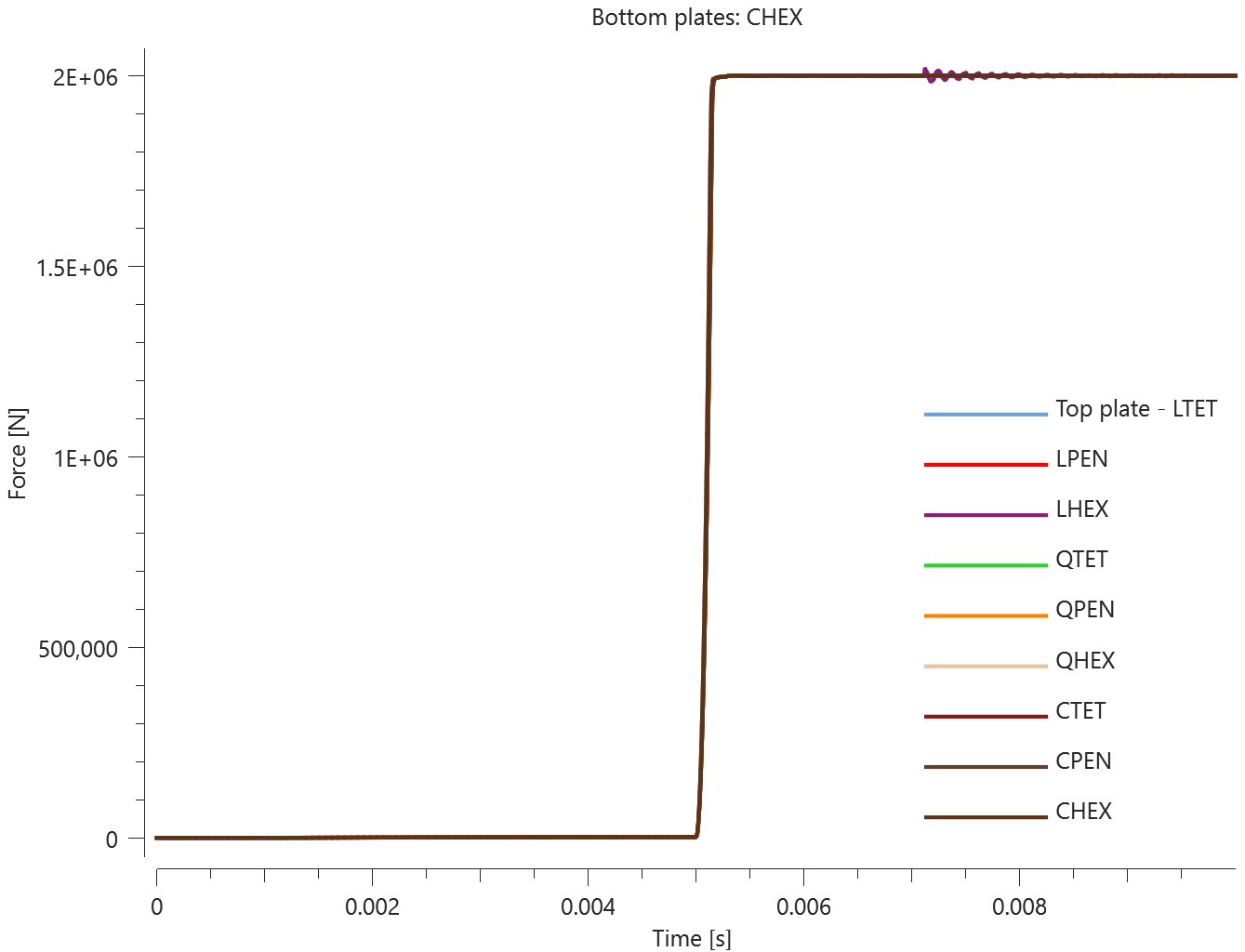
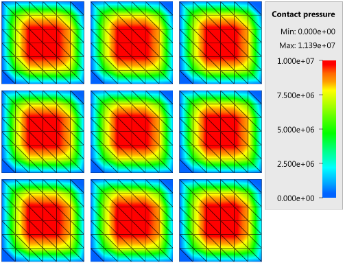
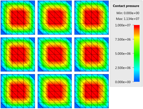
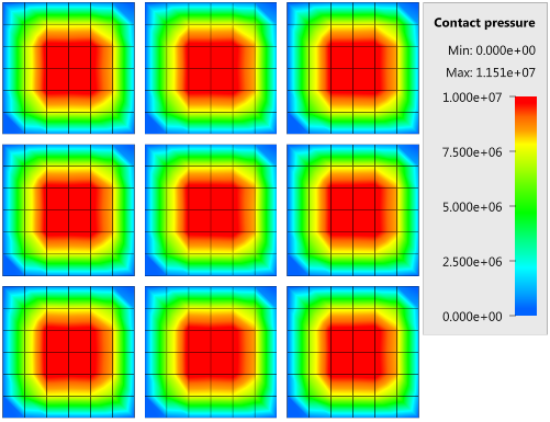
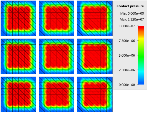
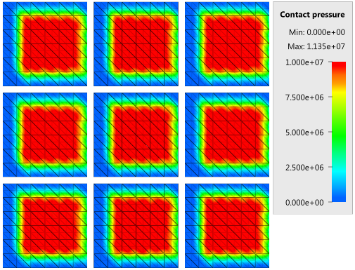
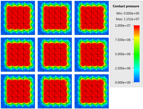
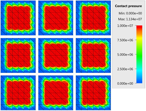
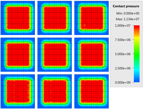
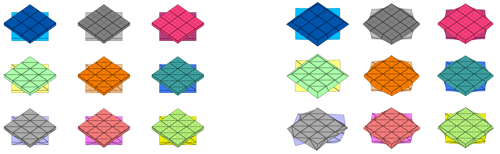
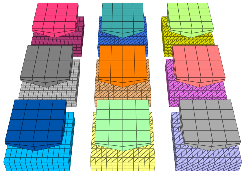
The test consists of 81 plate-pairs divided into nine models with nine plate-pairs in each model. One of the nine models is presented in Figure 1. The nine bottom plates in each model are of the same element type, but the type differs between the nine models. Each of the nine top plates consists of a unique type of elements and are the same in all models.
The type of elements used in the bottom plates in each model is presented in Table 1. Each row of top plates consists of a certain element type and each column of elements of a certain polynomial order. Top to bottom: tetrahedrons, pentahedron, hexahedron. Left to right: linear, quadratic, cubic.
| Model | Element type | |
|---|---|---|
| 1 | Linear tetrahedron | (LTET) |
| 2 | Linear pentahedron | (LPEN) |
| 3 | Linear hexahedron | (LHEX) |
| 4 | Quadratic tetrahedron | (QTET) |
| 5 | Quadratic pentahedron | (QPEN) |
| 6 | Quadratic hexahedron | (QHEX) |
| 7 | Cubic tetrahedron | (CTET) |
| 8 | Cubic pentahedron | (CPEN) |
| 9 | Cubic hexahedron | (CHEX) |
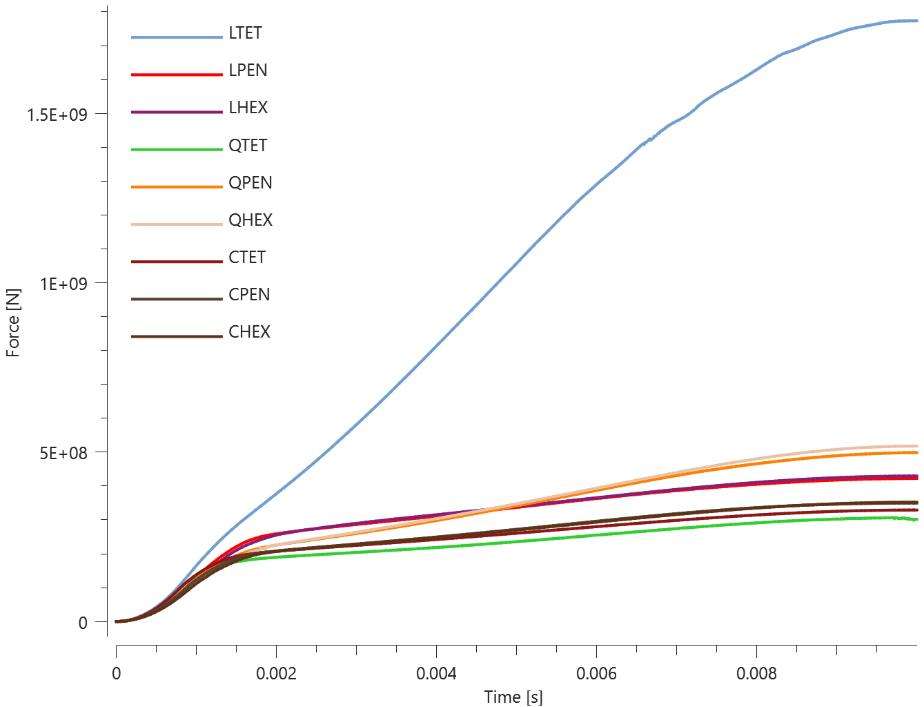
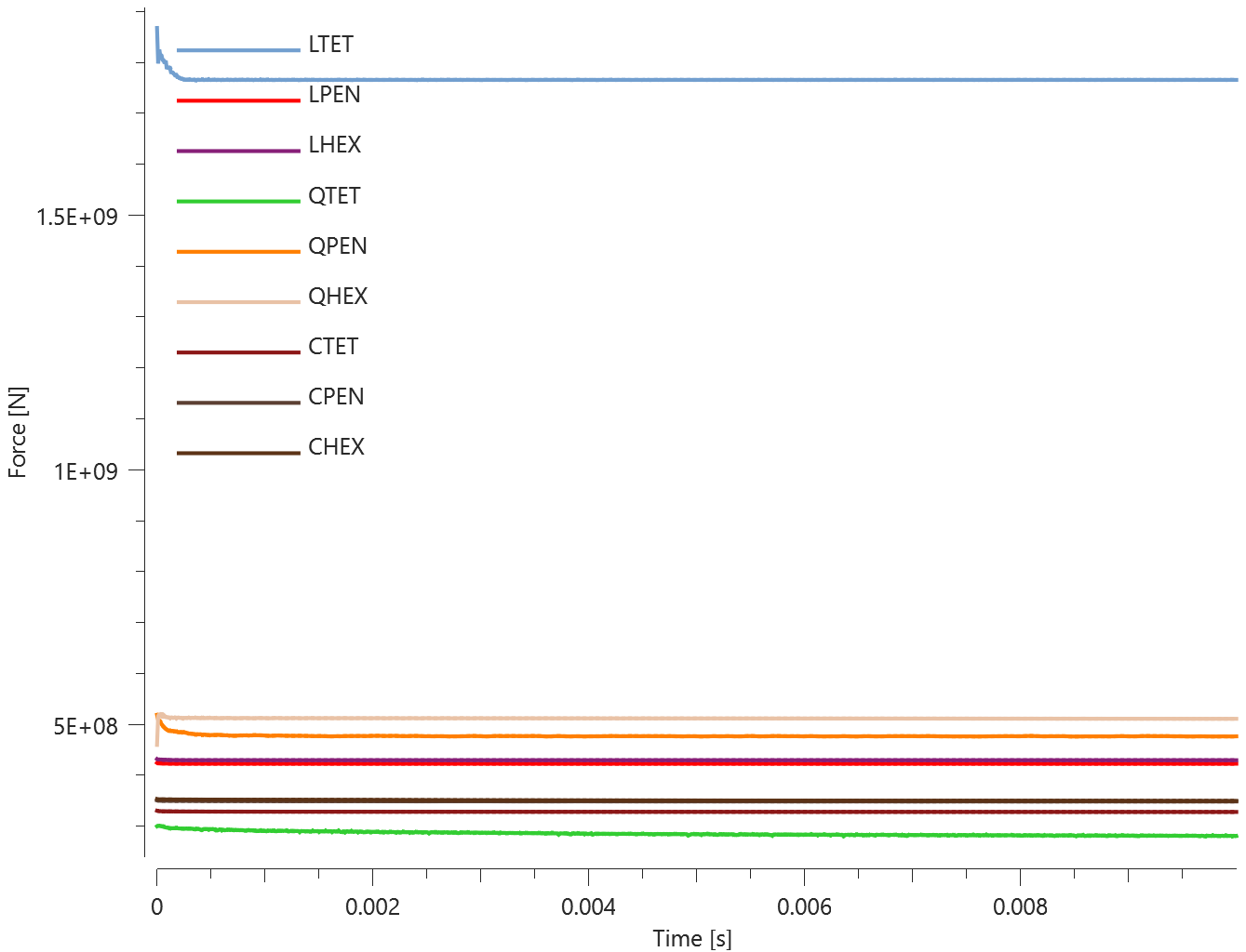
The plates are first pressed together by a prescribed pressure (*LOAD_PRESSURE) and then a prescribed motion (*BC_MOTION) is causing the top plates to slide against the fixed bottom plates.
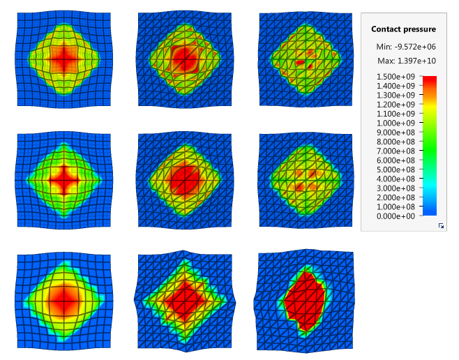
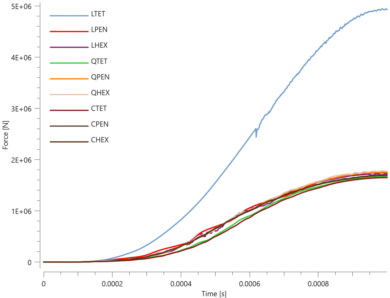
The contact force in the direction of the applied pressure vs. time for all plate-pairs and all models are presented in Figure 2 - 10 while the contact force in the sliding direction vs. time for all plate-pairs and all models are presented in Figure 11 - 19. Contour plots of the contact pressure for all models are presented in Figure 20 - 28
The contact forces are checked at termination.


Tests
This benchmark is associated with 9 tests.
Continue from state-file
"Optional title"
coid, accuracy_level, accuracy_edge
entype${}_1$, enid${}_1$, entype${}_2$, enid${}_2$, $\mu$, $pfac$, $t_{beg}$, $t_{end}$
merge, $\xi$, gid${}_0$, gid${}_1$, $\delta_{0}^{offset}$, $\delta_{0}^{max}$, $\delta^{edge}$
fid${}_{wear1}$, fid${}_{wear2}$, fid${}_{thermal}$, $\alpha_{edge}$, one_way, no_internal, $\sigma_{stick}$, fric_heat
The contact force in a simulation based on a state-file is verified in this test.
Tested parameter: $pfac$ (automatic calculation of penalty stiffness).
The model consists of nine pairs of plates. Each pair consists of a certain type of solid elements: LTET, LPEN, LHEX, QTET, QPEN, QHEX, CTET, CPEN or CHEX.
The process is divided into two steps. In step 1, the two plates in each pair are pressed together by a prescribed motion. At termination, the results are exported to a state-filek. The model at initiation and termination is displayed in Figure 1.
In step 2, the state-file is imported. The plates are fixed and a contact with the same configuration as in step 1 is defined. The contact force should therefore be of the same magnitude at termination of step 1, initiation of step 2 and at termination of step 2.
Contact forces in the direction of loading from step 1 and and step 2 are presented in Figure 2 and 3. The discrepancy in contact force between the different element types is mainly due to the coarse mesh that has been used. With a refined mesh, the discrepancy is reduced.
The contact forces are checked at initiation and termination in both steps.
Tests
This benchmark is associated with 2 tests.
Expanding spheres
"Optional title"
coid, accuracy_level, accuracy_edge
entype${}_1$, enid${}_1$, entype${}_2$, enid${}_2$, $\mu$, $pfac$, $t_{beg}$, $t_{end}$
merge, $\xi$, gid${}_0$, gid${}_1$, $\delta_{0}^{offset}$, $\delta_{0}^{max}$, $\delta^{edge}$
fid${}_{wear1}$, fid${}_{wear2}$, fid${}_{thermal}$, $\alpha_{edge}$, one_way, no_internal, $\sigma_{stick}$, fric_heat
Contact between multiple parts by using the "all-to-all"-option in *CONTACT is verified in this test.
Tested parameters: $entype_1$, $entype_2$ and $pfac$ (automatic calculation of penalty stiffness).
The model consists of 500 deformable spheres inside a rigid casing. There is no initial contact between the spheres, but the spheres are expanding during the course of the simulation, and contact emerges between the spheres. See Figure 1.

Maximum contact penetration, contact area at termination and energy balance are checked for version control.
Tests
This benchmark is associated with 1 tests.
Friction work to heat
"Optional title"
coid, accuracy_level, accuracy_edge
entype${}_1$, enid${}_1$, entype${}_2$, enid${}_2$, $\mu$, $pfac$, $t_{beg}$, $t_{end}$
merge, $\xi$, gid${}_0$, gid${}_1$, $\delta_{0}^{offset}$, $\delta_{0}^{max}$, $\delta^{edge}$
fid${}_{wear1}$, fid${}_{wear2}$, fid${}_{thermal}$, $\alpha_{edge}$, one_way, no_internal, $\sigma_{stick}$, fric_heat
Tested parameters: fric_heat.
This is a general test for *CONTACT. The model tests friction to heat conversion which is generated when a block is sliding against a plate.
The test setup is displayed in Figure 1
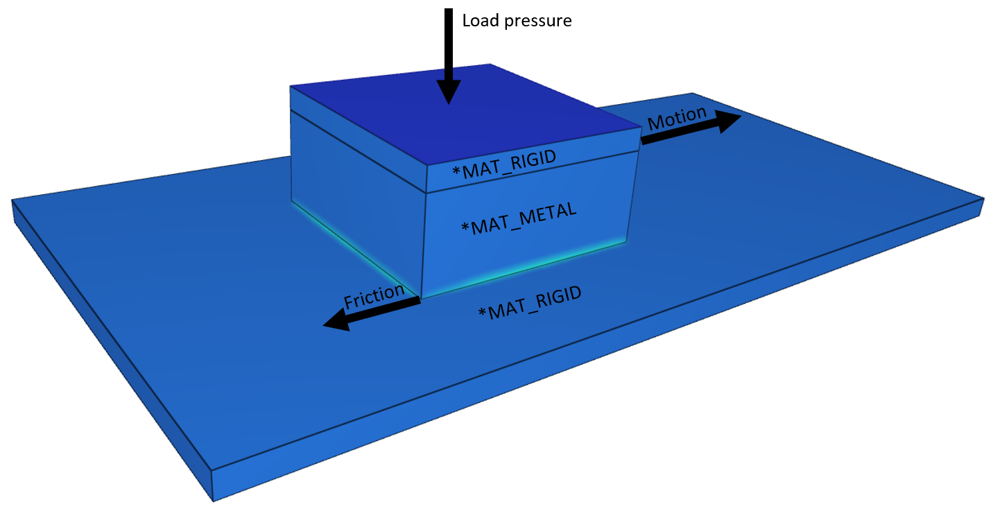
Targets:
The friction energy generated should be equal to the thermal energy that is added to the block and the plate.
First, average and last values for thermal energy and friction energy is checked for version control.
Tests
This benchmark is associated with 1 tests.
Newtons cradle
"Optional title"
coid, accuracy_level, accuracy_edge
entype${}_1$, enid${}_1$, entype${}_2$, enid${}_2$, $\mu$, $pfac$, $t_{beg}$, $t_{end}$
merge, $\xi$, gid${}_0$, gid${}_1$, $\delta_{0}^{offset}$, $\delta_{0}^{max}$, $\delta^{edge}$
fid${}_{wear1}$, fid${}_{wear2}$, fid${}_{thermal}$, $\alpha_{edge}$, one_way, no_internal, $\sigma_{stick}$, fric_heat
This is a general test for *CONTACT.
Tested parameter: $pfac$ (automatic calculation of penalty stiffness).
A Newton's cradle containing three balls is simulated in this test. The model is displayed in Figure 1. The collisons are elastic and no energy loss occurs in the system.
The energy balance, and maximum and minimum kinetic energy of the balls are checked.
Tests
This benchmark is associated with 1 tests.
Vickers hardness test
"Optional title"
coid, accuracy_level, accuracy_edge
entype${}_1$, enid${}_1$, entype${}_2$, enid${}_2$, $\mu$, $pfac$, $t_{beg}$, $t_{end}$
merge, $\xi$, gid${}_0$, gid${}_1$, $\delta_{0}^{offset}$, $\delta_{0}^{max}$, $\delta^{edge}$
fid${}_{wear1}$, fid${}_{wear2}$, fid${}_{thermal}$, $\alpha_{edge}$, one_way, no_internal, $\sigma_{stick}$, fric_heat
This is a general test for *CONTACT.
Tested parameters: $pfac$ (automatic calculation of penalty stiffness).
This is a model of a Vickers hardness test. The test is done with nine specimens, each modeled with a unique type of solid elements. The indenter is modeled with LHEX-elements in all cases, since negligible deformations are expected in the indenter. The specimen configuration is presented in Figure 1 and the maximum contact pressure is presented in Figure 2.
Contact forces vs. time are presented in Figure 3. Similar response is obtained from all specimens except for the linear tetrahedron specimen, which shows a significantly stiffer response.
Maximum contact force, maximum contact penetration and energy balance are checked.
Tests
This benchmark is associated with 1 tests.
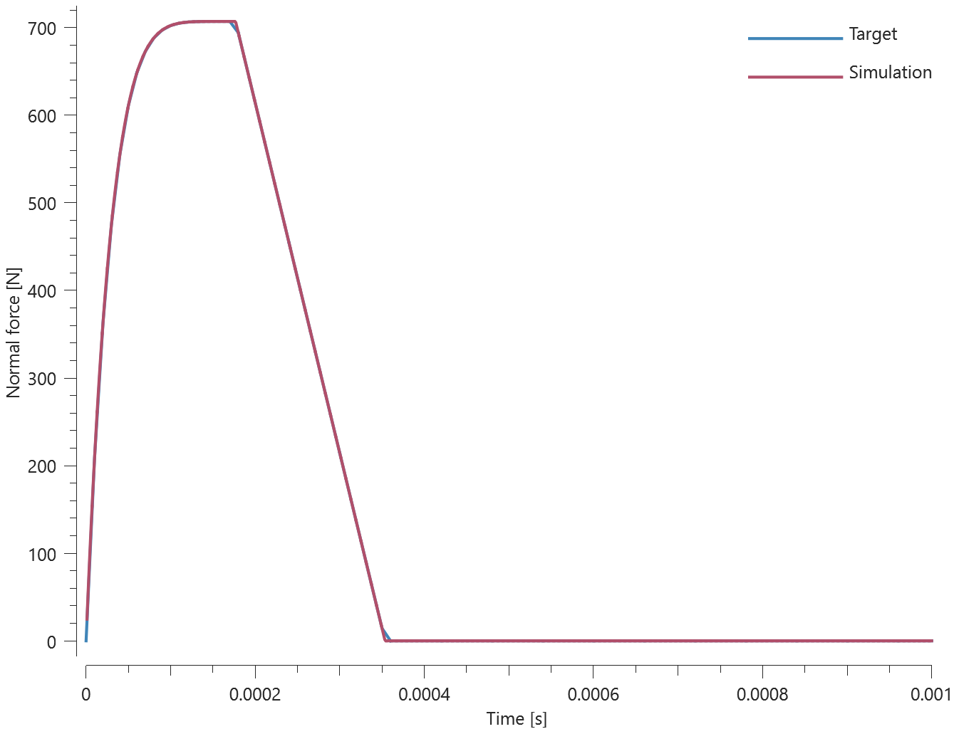
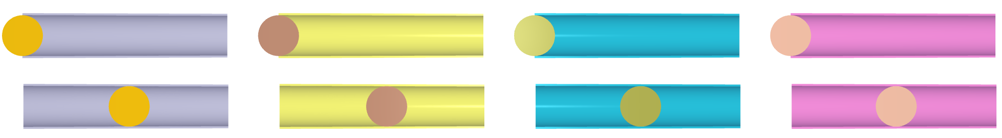
*CONTACT_ACCURACY
Accuracy edge
"Optional title"
coid, entype, enid, accuracy_level, accuracy_edge
Accuracy edge in *CONTACT_ACCURACY is verified in this test.
Tested parameters: accuracy_edge.
Two identical sets consisting of a cube and a cylinder are used in this test. The cylinders are linearly tapered, and the inner radius at one end equals the cubes face diagonal, $D_c/2$, while the radius on the other end equals $0.97\cdot D_c/2$.
The cubes are positioned inside the cylinders, so that only edges are in contact, and given an initial velocity so that they move towards the other sides of the cylinders. The test setup is displayed in Figure 1.
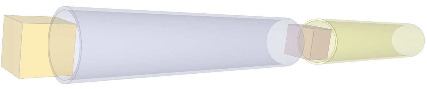
Contact forces between the cubes and the cylinders increases gradually as the cubes are moving down the cylinders. The smoothness of the contact forces are controlled with contact accuracy. The accuracy level used is 10 for both sets but the flag to activate increased accuracy at sharp edges (Accuracy_edge) is activated for the second set (right) but not for the first set(left). The initial and final state of the model is displayed in Figure 2.
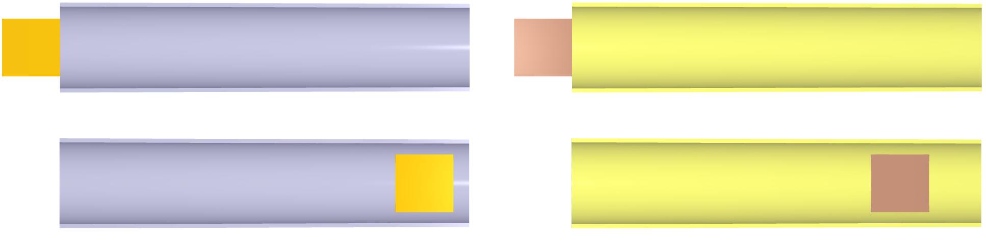
Contact force vs time for both sets is presented in Figure 3.
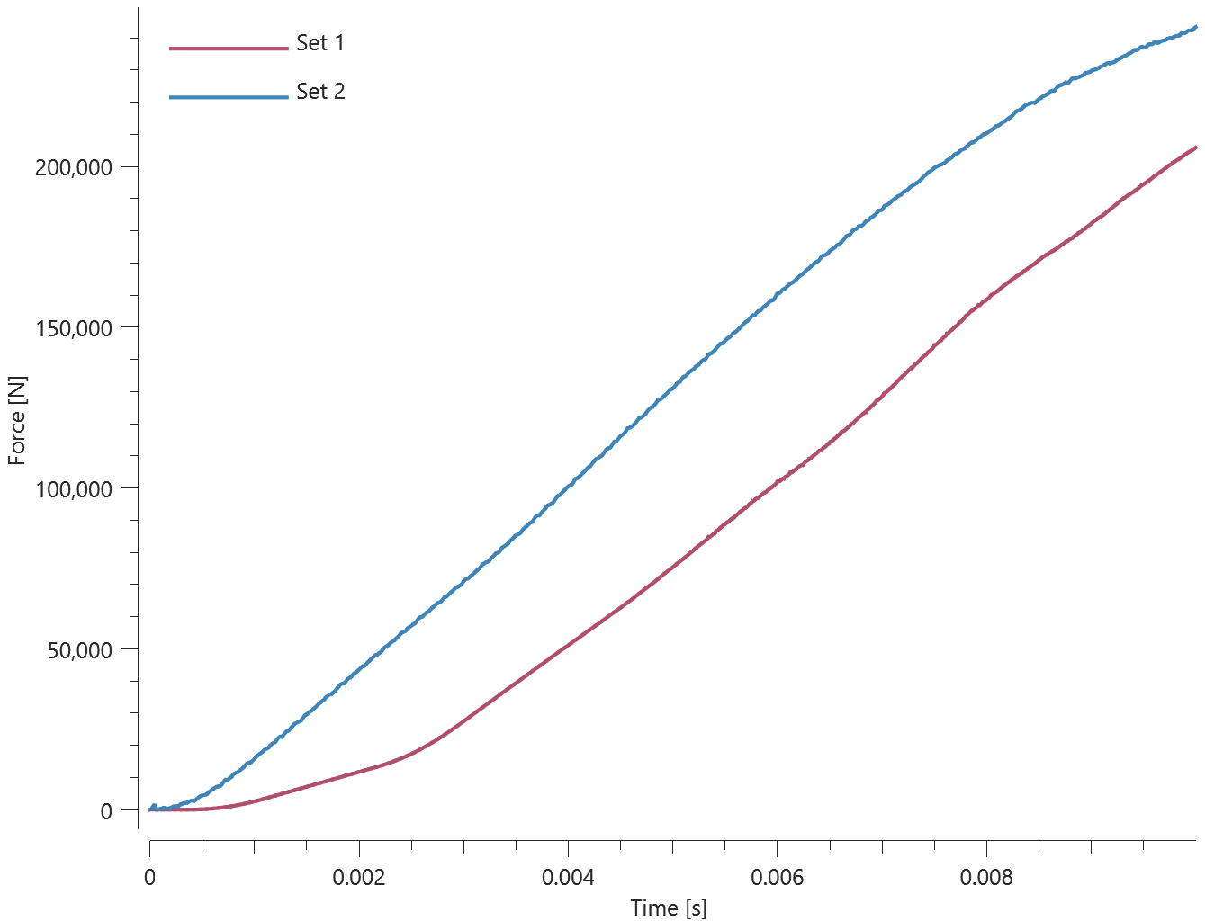
As seen in Figure 3, Accuracy_edge when activated leads to increased contact force.
Maximum and average contact force is checked for both sets.
Tests
This benchmark is associated with 1 tests.
Accuracy level
"Optional title"
coid, entype, enid, accuracy_level, accuracy_edge
Contact accuracy level in *CONTACT_ACCURACY is verified in this test.
Tested parameters: accuracy_level.
Four identical sets consisting of a sphere and a cylinder are used in this test. The cylinders are linearly tapered, and the inner radius at one end equals the sphere radius, $R_s$, while the radius on the other end equals $0.97\cdot R_s$.
The spheres are positioned inside the cylinders, at the end with a radius $R_s$, and given an initial velocity so that they move towards the other end of the cylinder. The initial and final state of the model is displayed in Figure 1.
Contact forces between the spheres and the cylinders increase gradually as the spheres moves down the cylinder, and the smoothness of the contact forces are controlled by the contact accuracy. Investigated accuracy levels are 1, 2, 3 and 10 for set 1, 2, 3 and 4, respectively.
Contact force vs time for each set is presented in Figure 2.
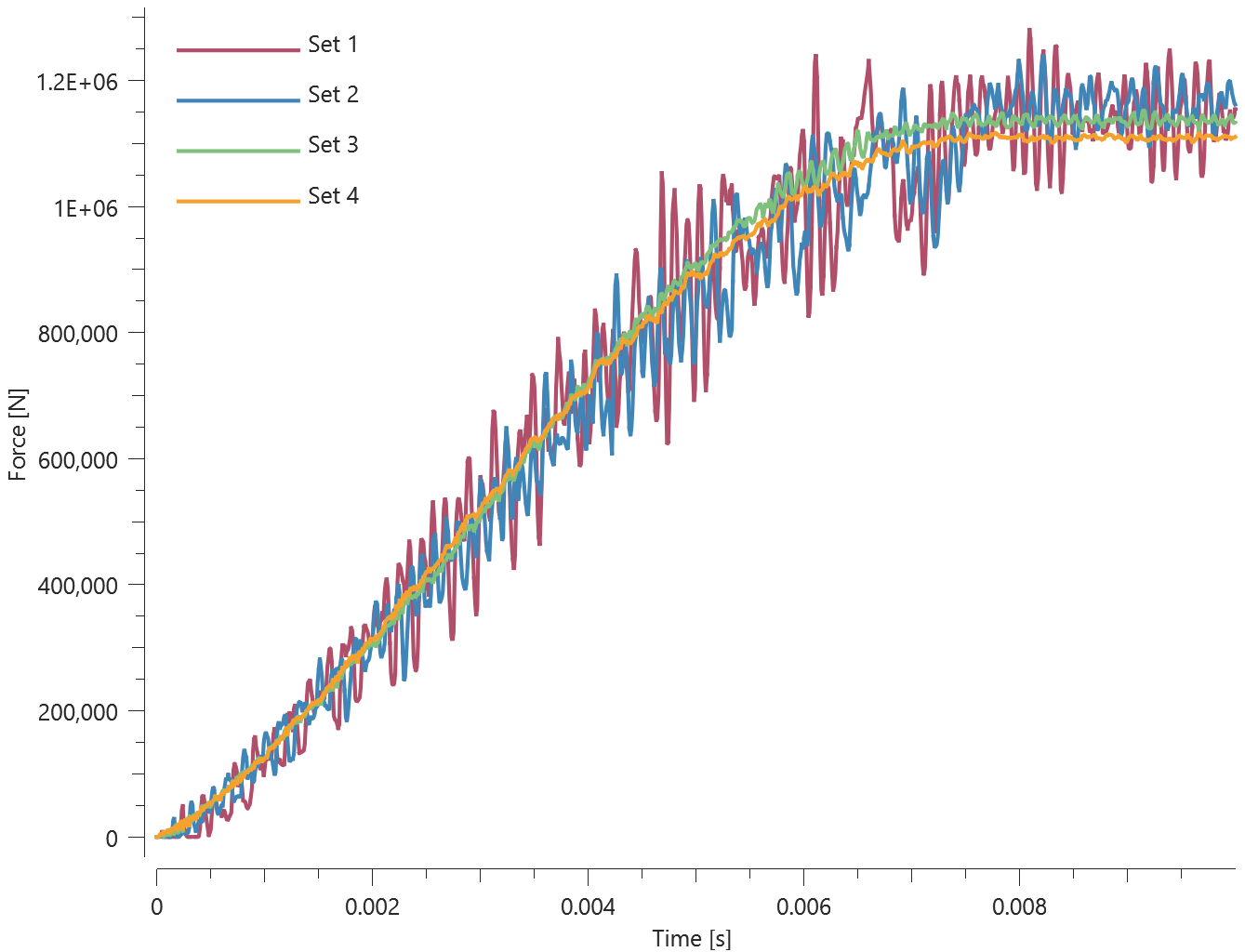
Quantifying the "noise" of the contact force in set 1, 2 and 3 is done by integrating the absolute value of the difference between contact force in set 1, 2, 3 and the contact force of set 4, meaning that contact force in set 4 acts as reference curve. The accumulated noise of set 1, 2, 3 is presented in Figure 3.
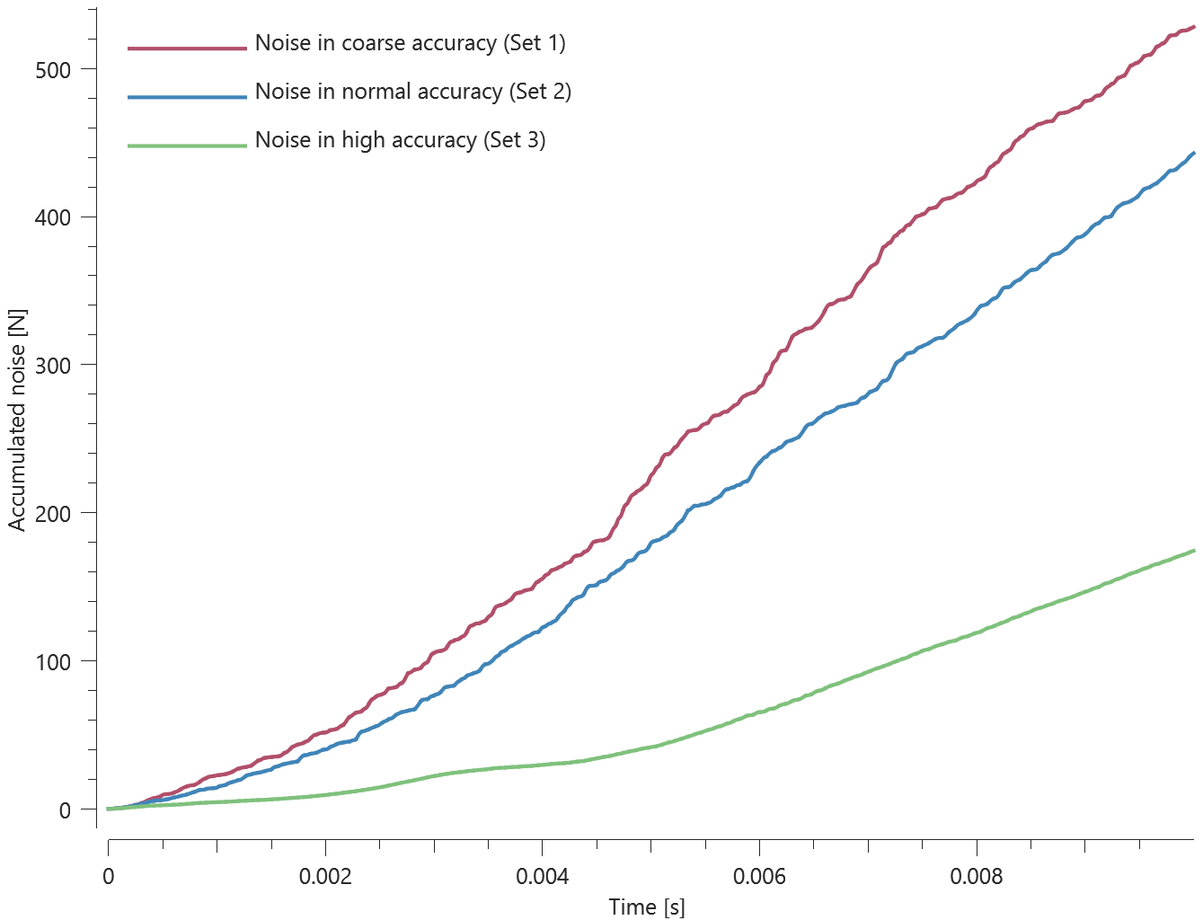
As seen in Figure 3 , a higher contact accuracy leads to reduced level of noise.
Maximum and average contact force in set four is checked together with maximum and average accumulated noise in set 1, 2 and 3.
Tests
This benchmark is associated with 1 tests.
*CONTACT_REBAR
Contact between rebars and elements
"Optional title"
switch
The command *CONTACT_REBAR is tested. The command is used to define contact between rebars and the "regular" FE-elements. Five boxes (*COMPONENT_BOX) and five rebars (*COMPONENT_REBAR) are used in the test, see Figure 1.
The rebars are at rest at initiation whereas a prescribed velocity of 10 m/s is imposed on the boxes (towards the rebars). The boxes impacts the rebars and the kinetic energy of each rebar at termination is checked for version control. The largest contact penetration is also checked.
Tests
This benchmark is associated with 1 tests.
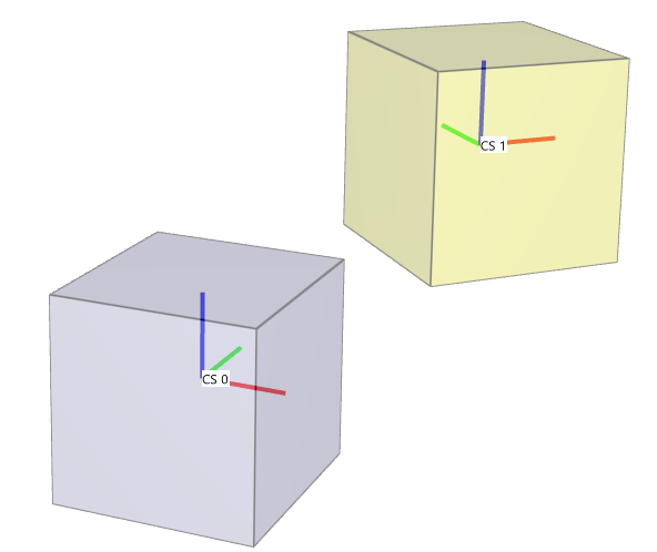
*COORDINATE_SYSTEM
Position
"Optional title"
csysid, $x_0$, $y_0$, $z_0$, pid
$\hat{x}_x$, $\hat{x}_y$, $\hat{x}_z$, $\bar{y}_x$, $\bar{y}_y$, $\bar{y}_z$
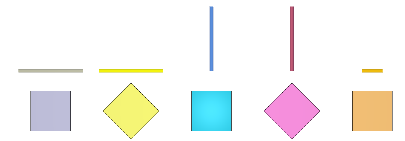
This model tests the *COORDINATE_SYSTEM command. Three identical cubes are created with side length 1. Cube 1 is created with a fixed coordinate system while the other cubes are created with a tilted coordinate system with its origin located on the boundary between them. The coordinate system is given an optional part ID of 3 which ties it to cube 3. The cubes are set in motion and as cube 3 separates from cube 2, the coordinate system is forced to follow cube 3 while the fixed coordinate system remains at its initial location. See Figure 1.
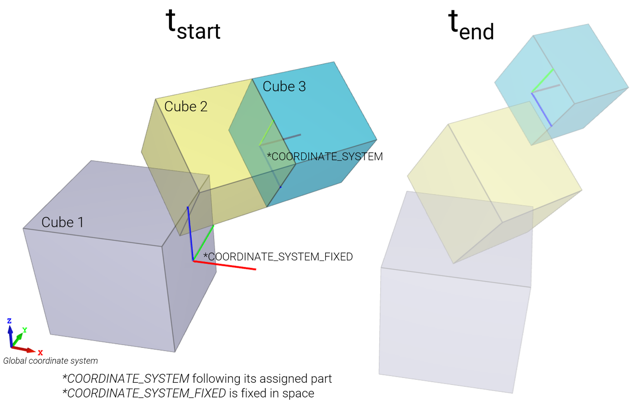
The final positions of the coordinate systems are checked in the version control.
Tests
This benchmark is associated with 1 tests.
*COORDINATE_SYSTEM_CYLINDRICAL
Transform mesh
"Optional title"
csysid, $x_0$, $y_0$, $z_0$
$\hat{z}_x$, $\hat{z}_y$, $\hat{z}_z$, $\hat{R}_{0x}$, $\hat{R}_{0y}$, $\hat{R}_{0z}$
This tests the *COORDINATE_SYSTEM_CYLINDRICAL command. This command is used with *TRANSFORM_MESH_CYLINDRICAL to transform a mesh with defined cylindrical coordinates. The model is a pipe. In the transformation, inner and outer radius are decreased and the model is translated in the axial direction. Final coordinates of two nodes at opposite ends are checked for version control. One is at the inner radius, the other at the outer radius.
Tests
This benchmark is associated with 1 tests.
*COORDINATE_SYSTEM_FIXED
Positioning test & transform mesh
"Optional title"
csysid, $x_0$, $y_0$, $z_0$
$\hat{x}_x$, $\hat{x}_y$, $\hat{x}_z$, $\bar{y}_x$, $\bar{y}_y$, $\bar{y}_z$
This model tests the *COORDINATE_SYSTEM_FIXED command. Two elements are created, one at the center of the global coordinate system and one at the center of a fixed, local coordinate system. The latter system is shifted one unit along all axis and the direction of the X-axis in the global coordinate system has the unit vector ($1,1,0$). It is therefore at a 45° angle in the XY-plane relative to the global system.
The center of the cubes are at origin of their respective coordinate systems, with side lengths of 1 unit. Node 1 of the first cube should thus have coordinates ($-0.5,-0.5,-0.5$). The corresponding node of the second cube, node 9, should have coordinates ($1,0.5,1-\sqrt {0.5}$). This is checked in the version control.
Tests
This benchmark is associated with 2 tests.
*COORDINATE_SYSTEM_FUNCTION
Coordinate system defined with functions
"Optional title"
csysid, $x_0$, $y_0$, $z_0$
$\hat{x}_x$, $\hat{x}_y$, $\hat{x}_z$, $\bar{y}_x$, $\bar{y}_y$, $\bar{y}_z$
Tested parameters : csysid, $x_0$, $y_0$, $z_0$, $\hat{x}_x$, $\hat{x}_y$, $\hat{x}_z$, $\bar{y}_x$, $\bar{y}_y$, $\bar{y}_z$.
This model tests the command *COORDINATE_SYSTEM_FUNCTION. A local coordinate system with its origin following sensor ID=1 and with prescribed, time dependent, direction cosines. It is rotating 360° around its Z-axis for the time duration.
A cube with side length $1 \ m$ is given a prescribed displacement of $1 \ m$ in the global X-direction. The local coordinate system is used as a translational constraint for the cube, restricting its motion in the current local Y- and Z-axis. Hence, the cube will only translate in the local coordinate system's current X-direction. See Figure 1.
The displacement of the cube is displayed in Figure 2 together with target curves from a verification script.
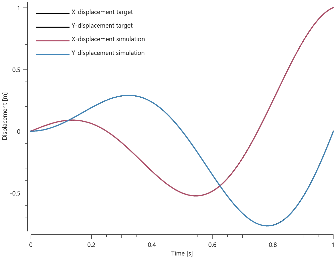
Final translation should be $1 \ m$ in the global X-direction. The position of the cube is checked for version control.
Tests
This benchmark is associated with 1 tests.
*COORDINATE_SYSTEM_NODE
Torque
"Optional title"
csysid, N${}_1$, N${}_2$, N${}_3$
This tests the *COORDINATE_SYSTEM_NODE command. A metal box has a rigid box merged to it at one end. A constant force is applied to the rigid body with *LOAD_FORCE. This force is defined in a node coordinate system so as to always act perpendicular to the length of the model. It thus acts as a torque on the box.
At the opposite end, in the plane of the applied force, the corner nodes are constrained in all directions such that the box can only rotate about the z-axis. The torque is parallel to the Z-axis, in the opposite direction ($\mathbf{-z} \parallel \textbf{r} \times \mathbf{F}$).
The spin of the rigid body about the Z-axis should therefore decrease linearly. See Figure 1. This is checked for version control.
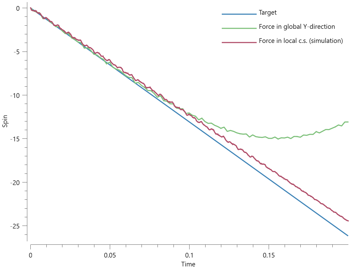
Tests
This benchmark is associated with 1 tests.
*COUPLING_REBAR
Verification test
"Optional title"
coid
entype${}_r$, enid${}_r$, entype${}_c$, enid${}_c$, keep
This benchmark is a verification of the *COUPLING_REBAR command. The simulation model used can be found in the command manual example.
A rebar cage is embedded in a circular concrete slab. COUPLING_REBAR is here used to trim (delete) rebar elements outside the slab.
Checks are added for the rebar mass at the start and end of the simulation.
*CURVE
Displacements set with curve
"Optional title"
cid, $sf_{\mathrm{x}}$, $sf_{\mathrm{y}}$, type${}_{\mathrm{x}}$, type${}_{\mathrm{y}}$
$x_1$, $y_1$
.
$x_{\mathrm{n}}$, $y_{\mathrm{n}}$
This tests the *CURVE command. Three rigid elements are moved by the *BC_MOTION command. All motion is defined by displacement set by *CURVE inputs. One element follows a simple linear trajectory before returning to initial position, while the two other elements follows trajectories that have scaled abissa or ordinate values. Displacement of elements are checked for version control.
Tests
This benchmark is associated with 1 tests.
*DEFINE_ELEMENT_SET
Change element type in impact zone
"Optional title"
coid
entype, enid, fid, padding
Tested parameters: coid, entype, enid, fid, padding.
This model tests the command *DEFINE_ELEMENT_SET. It consists of two steps.
A cylindrical impactor punches a hole in a plate. The model is first run with only linear elements (Step 1). The purpose of this step is to identify the region undergoing large deformations. This is done by formulating an inclusion criteria by setting a FUNCTION (here defined as elements with effective plastic strains larger than 0.5).
$$ epsp - 0.5 $$
The FUNCTION is evaluated for each element in the part. An element will be included in the part set if the function returns a positive value. At termination, the element set is written to the file element_set_X.k, (where X=coid) which will be used in step 2.
In subsequent simulations (Step 2) elements in the set are converted to 3rd order hexahedra (for increased accuracy). To test the paramater padding, two element sets are generated, one with and one without padding. See Figure 1.
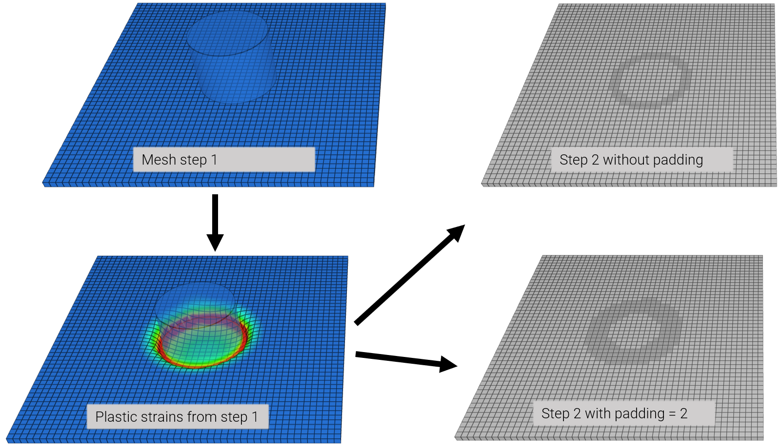
The element sets generated are checked for version control.
Tests
This benchmark is associated with 3 tests.
*ELEMENT_SHELL
Contact
eid, pid, nid${}_1$, nid${}_2$, nid${}_3$, nid${}_4$
This tests the contact interference of *ELEMENT_SHELL and other deformable bodies. *ELEMENT_SHELL can only be used to generate rigid bodies. The element thickness is specified in *PART, but this thickness is not active in contact situations.
The set-up is a rigid cone with an initial velocity impacting at the center of the open face of a pipe. The pipe has a lesser radius than the cone, bringing the cone to halt. The initial kinetic energy of the cone is $1585.5 \ kJ$ ($m = 317.1 \ kg$ , $v_{0} = 100 \ m/s$), and this value is checked against the final energy balance found in "energy.out".
Note that by using linear elements in the first test, the stiffness is artificially high. This offset is improved in the second and third run, in which quadratic and cubic elements are used.
Tests
This benchmark is associated with 3 tests.
Volume and mass verification
eid, pid, nid${}_1$, nid${}_2$, nid${}_3$, nid${}_4$
This tests that *ELEMENT_SHELL and *PART generates elements correctly. Mass and volume of a $1 \ m$ square rigid shell with a thickness of $1 \ m$ is checked in part.out. The density of the material is $1000 \ kg/m^3$. The generated shell element can be seen in Figure 1.
Tests
This benchmark is associated with 1 tests.
*ELEMENT_SOLID
Higher order elements
eid, pid, nid${}_1$, nid${}_2$, nid${}_3$, nid${}_4$, nid${}_5$, nid${}_6$, nid${}_7$, nid${}_8$
This tests the higher order *ELEMENT commands. This includes quadratic and cubic hexahedron, pentahedron, and tetrahedron elements - six element types in total (Figure 1 to 6.). The pentrahedron elements can be oriented in two different ways, both are tested for both the quadratic and cubic element.
The element mesh has been created using *ELEMENT_SOLID and *CHANGE_P-ORDER and then exported to an input file that has the higher order *ELEMENT commands. In these tests, these input files are checked using *BC_MOTION. The geometry is a block with side length of $0.01 m$. It is stretched in Z-direction with a logarithmic strain of 1. Hardening of material is Ramberg Osgood ($n=1, K= 150e^{9}$). The yield strengh is $300 MPa$, Young's modulus is $210 GPa$, and Poisson's ratio is $0.33$.
Stress and strain at the end of the simulation is checked for version control.
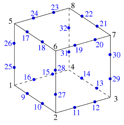
Tests
This benchmark is associated with 8 tests.
Linear elements
eid, pid, nid${}_1$, nid${}_2$, nid${}_3$, nid${}_4$, nid${}_5$, nid${}_6$, nid${}_7$, nid${}_8$
This tests the *ELEMENT_SOLID command. This includes linear hexahedron, pentahedron and tetrahedron elements. In these tests, the elements are checked using *BC_MOTION. The geometry is a block with side length of $0.01 m$. It is stretched in Z-direction with a logarithmic strain of 1. Hardening of material is Ramberg-Osgood ($n = 1, K = 150e^{9}$). The yield strength is $300 MPa$, Young's modulus is $210 GPa$, and Poisson's ratio is $0.33$.
For version control, stress and strain is checked at the end of simulation.
Tests
This benchmark is associated with 4 tests.
*END
End input
This model tests the *END command. The test is identical to the test "*LOAD_GRAVITY - Gravity test", with the addition of an *INITIAL_VELOCITY command after the *END command. If the *END command doesn't end the input correctly, the elements will output different velocities and the checks will fail.
Tests
This benchmark is associated with 1 tests.
*EOS_GRUNEISEN
Shock wave test
eosid, $S_1$, $\Gamma$, $L$, $p_{cut}$
$S_2$, $S_3$, $a$
Tested parameters: eosid, $S$, $\Gamma$.
This model tests the *EOS_GRUNEISEN command.
An abrupt pressure is introduced on one side of a highly elongated rectangular cuboid with dimensions:
Length = 1 m
Width = 0.001 m
Height = 0.001 m
As the shock wave travels along its length, 10 equally-distanced sensors are measuring pressure. The Mie-Gruneisen equation of state is implemented with the command *EOS_GRUNEISEN. For comparison one cuboid with *EOS_GRUNEISEN and one without it is tested for.
The test setup is displayed in Figure 1 and 2.
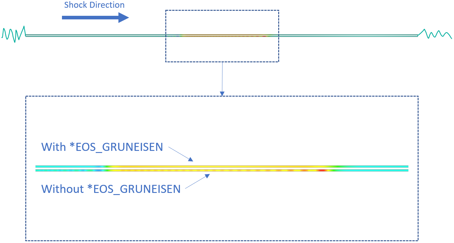
The wave induced by the shock pulse takes the shape of a square wave. This can be seen in Figure 3, where the difference between the two test cases is visble. Only two sensors are displayed for clarity.
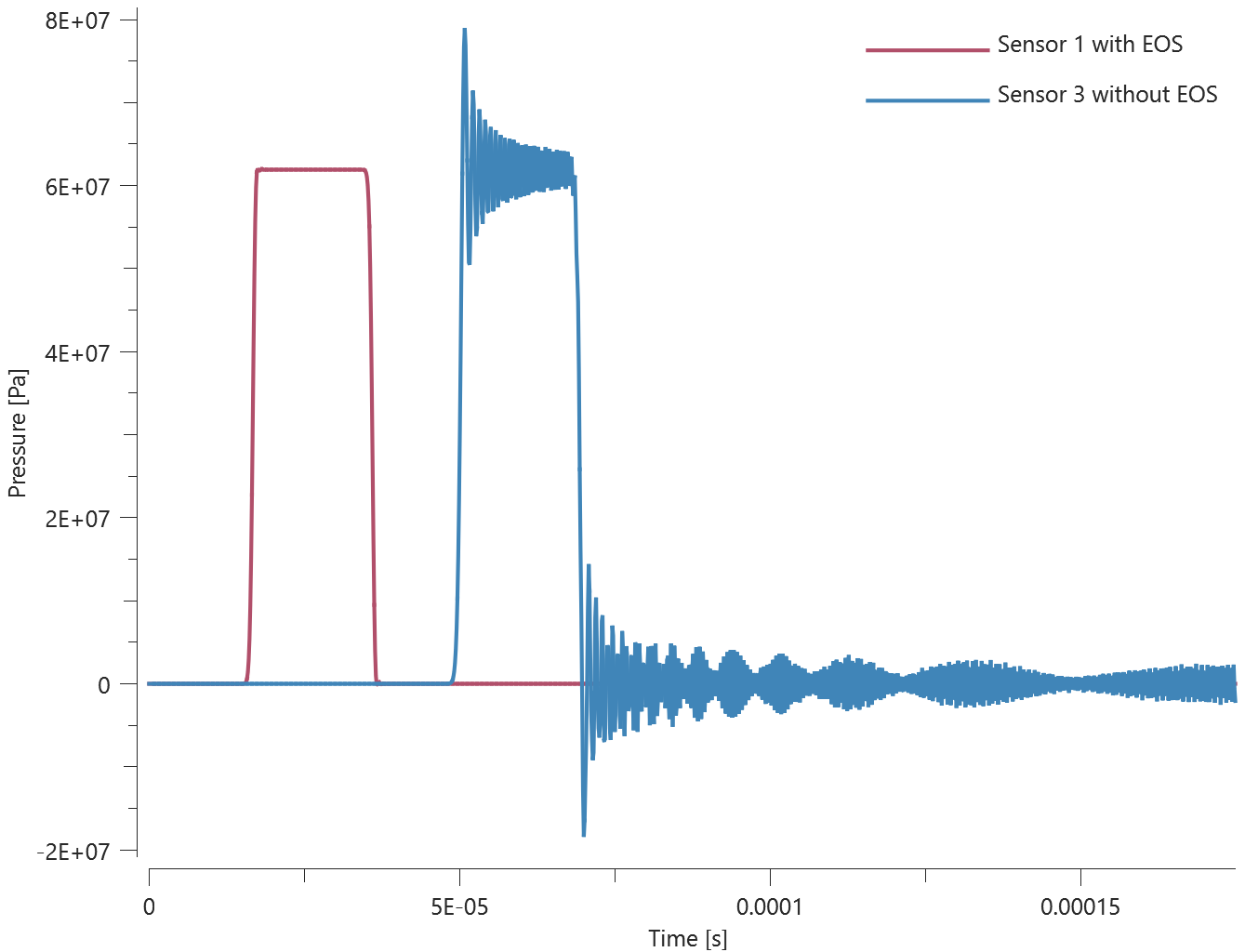
The noise is measured by integrating the absolute value of the pressure difference between the test cases at each sensor. See Figure 4.
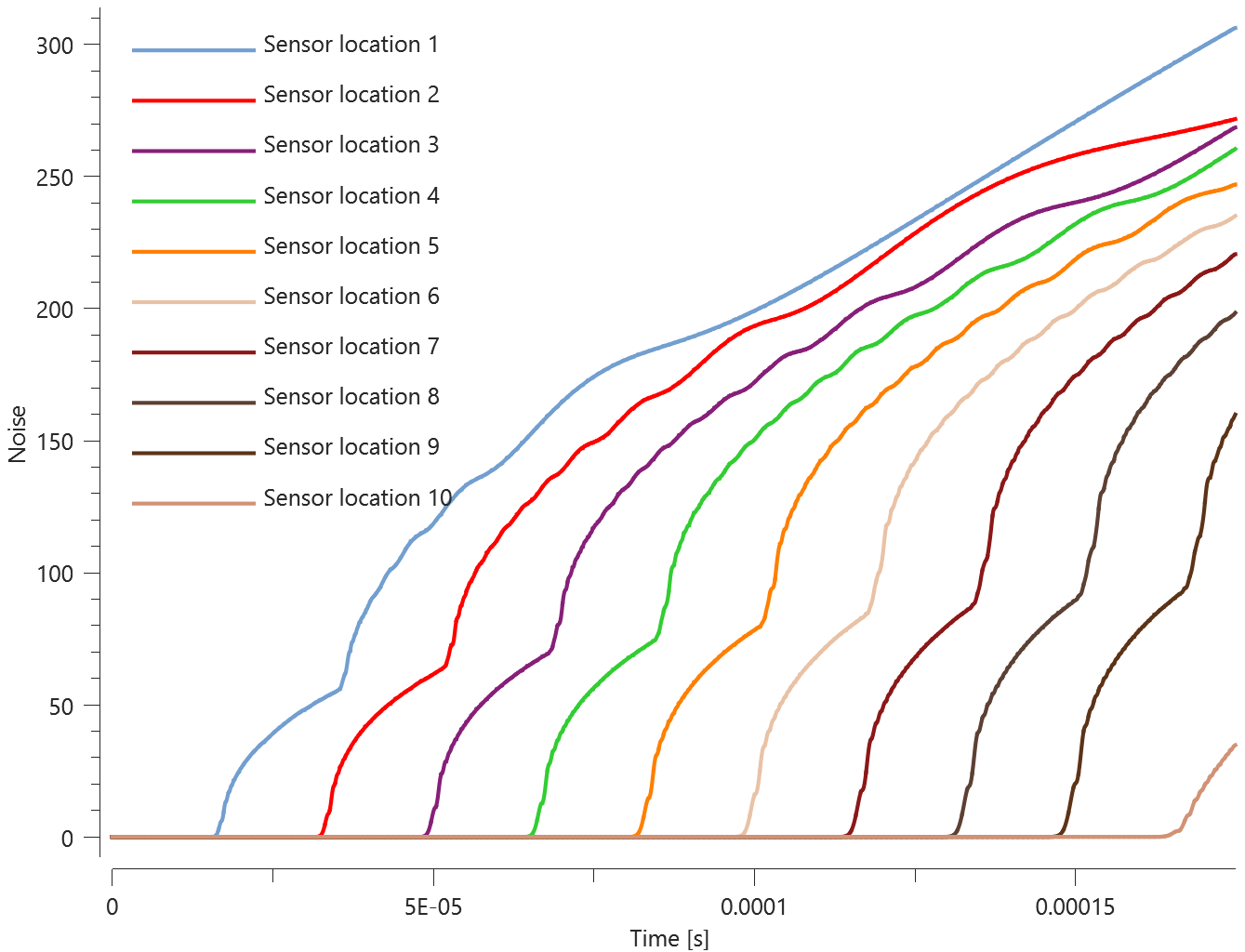
The maximum value of the pressure difference at each sensor is checked for version control.
Tests
This benchmark is associated with 1 tests.
*EROSION_CRITERION
Element erosion
coid
entype, enid, $\Delta t^{erode}$, $\varepsilon_{geo}^{erode}$, $\varepsilon_v^{erode}$, $\varepsilon_{eff}^{p,erode}$
This test is similar to the test "*PART - Element erosion". In this test, the erosion criteria are instead defined with *EROSION_CRITERION.
Tests
This benchmark is associated with 1 tests.
Priority test
coid
entype, enid, $\Delta t^{erode}$, $\varepsilon_{geo}^{erode}$, $\varepsilon_v^{erode}$, $\varepsilon_{eff}^{p,erode}$
This test is similar to the test "*EROSION_CRITERION - Element erosion". In this test, the erosion criteria are defined with *EROSION_CRITERION but also in *PART.
It is tested that the erosion parameters defined in *PART have higher priority.
Tests
This benchmark is associated with 1 tests.
*EROSION_CRITERION_SPH_DRIVEN
Fracture toughness specimen
"Optional title"
coid
pid, $D^{erode}$, $\varepsilon_{eff}^{p,erode}$, $R$
This test is a copy of the example given for *EROSION_CRITERION_SPH_DRIVEN in the command manual.
A model of a simple fracture toughness test specimen. Elements are eroded as the crack grows. Note that the SPH nodes have a residual strength even after reaching full damage (res_SPH). This prevents a local disintegration of the material along the crack.
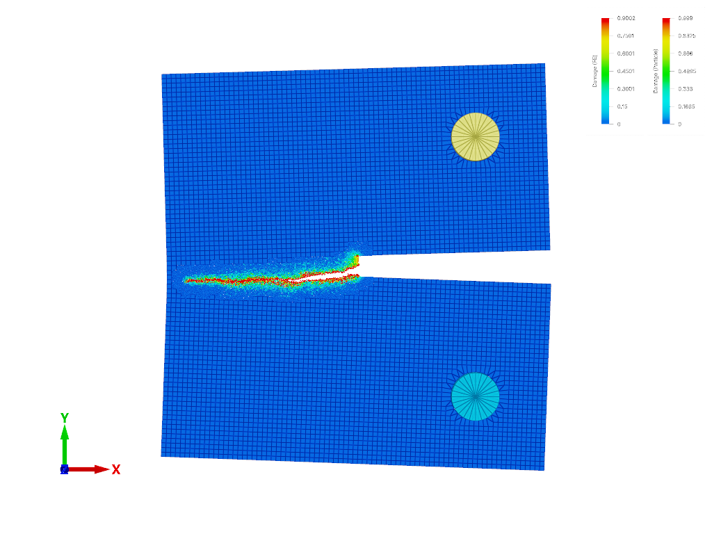
A SPH sensor is placed where the crack tip will be located at the end of the simulation. Checks are done for damage at first and last value in the sensor, as well as the total SPH subdomain mass. The checks are for version control.
Tests
This benchmark is associated with 1 tests.
*FREQUENCY_CUTOFF
Testing LOAD_DAMPING - Mass damping
"Optional title"
coid
entype, enid, $\Delta t_{target}$, $sf_{cap}$, $t_{start}$, $t_{end}$, no_regms
Tested parameters: coid, entype, enid, $\Delta t_{target}$.
This model tests the *FREQUENCY_CUTOFF command for the already existing test, See "LOAD_DAMPING - Mass damping".
The objective of this test is to speed up the simulation time without compromising accuracy. This is done by suppressing angular frequencies $w > 2/\Delta t_{target}$ which allows for larger time steps.
The target time step size is set to $\Delta t_{target} = 1\mu s$.
Tip displacement of the beams from the original test (without *FREQUENCY_CUTOFF) compared with this test (with *FREQUENCY_CUTOFF) can be seen in Figure 1
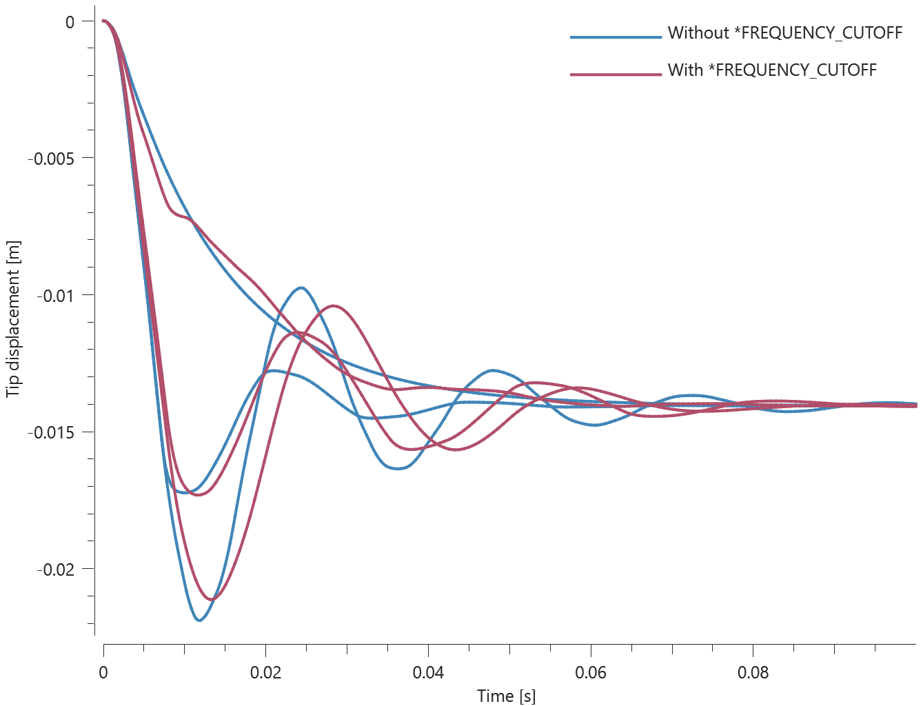
First, average, min and last values of tip displacements are checked for version control.
Tests
This benchmark is associated with 1 tests.
Testing MAT_METAL - Quasi-static yield stress
"Optional title"
coid
entype, enid, $\Delta t_{target}$, $sf_{cap}$, $t_{start}$, $t_{end}$, no_regms
Tested parameters: coid, entype, enid, $sf_{cap}$.
This model tests the *FREQUENCY_CUTOFF command for the already existing test, See "MAT_METAL - Quasi-static yield stress". The objective is to speed up the simulation time without compromising accuracy.
The primary purpose of the command is to allow for larger time steps in quasi-static processes. This is achieved by suppressing angular frequencies $\omega > 2/\Delta t_{target}$. The scale factor, $sf_{cap}$ which limits the maximum increase of time step size is set to 4.
Effective stress vs. effective plastic strain is presented in Figure 1 together with a target curve from a verification script.
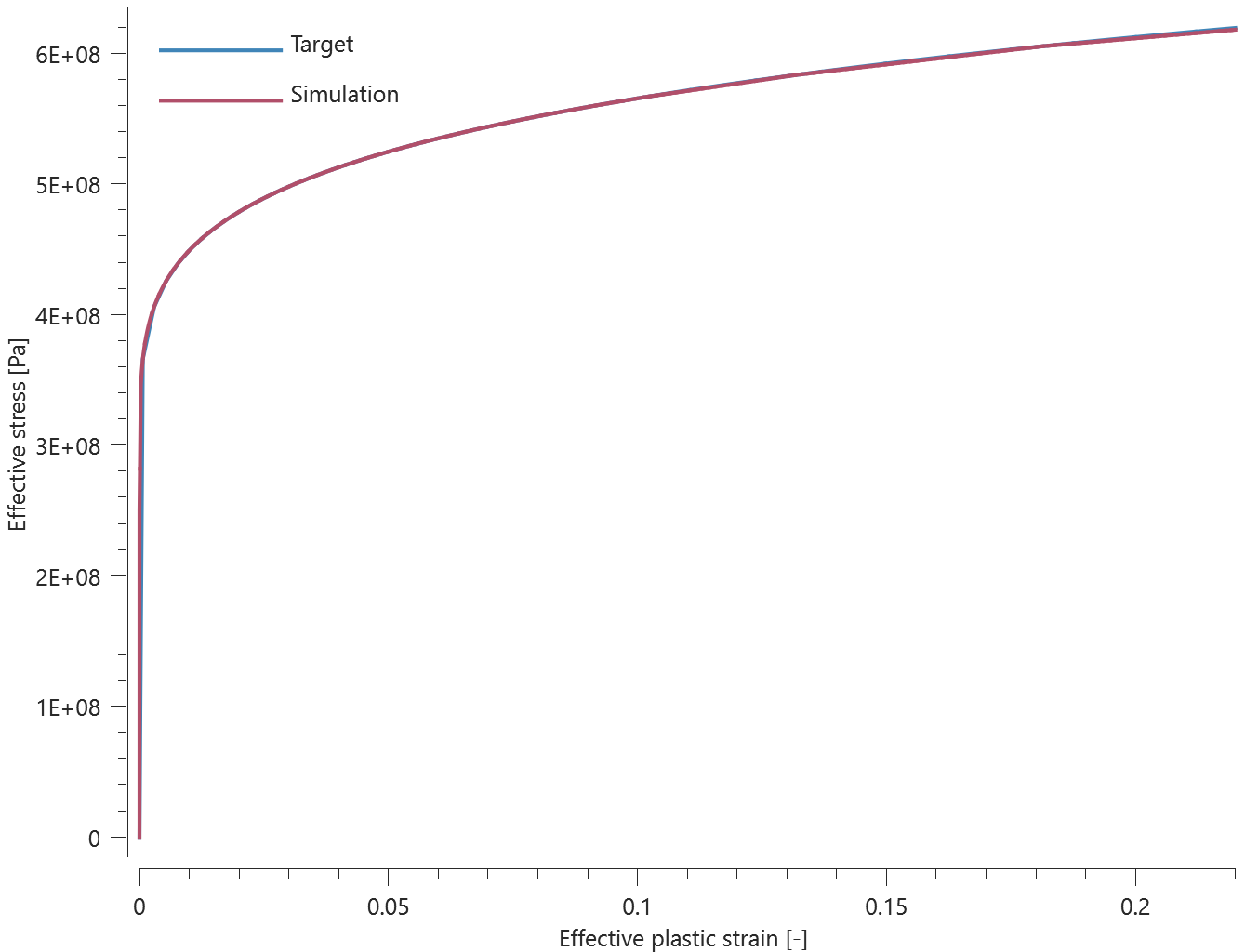
Maximum and average effective stress and effective plastic strain are checked for version control.
Tests
This benchmark is associated with 1 tests.
*FUNCTION
Basic functions
"Optional title"
fid, derivative, $f(0)$, $\dot{f}(0)$, type${}_{\mathrm{x}}$, type${}_{\mathrm{y}}$
expression
This tests the *FUNCTION command and some of its supported functions and parameters. More specifically, these built-in functions are tested:
- Trigonometric sine function
- Trigonometric cosine function
- Absolute value
- Minimum value of $x_{1},x_2...$ $x_n$
- Maximum value of $x_{1},x_2...$ $x_n$
- Step function ($x<0\Rightarrow0$, $x>0\Rightarrow1$)
- Sign function ($x<0\Rightarrow-1$, $x>0\Rightarrow1$)
- Exponential function ($e^x$)
- $x_{1},x_2...$ $x_n$ & $\bullet$ Square root function
- $x_{1},x_2...$ $x_n$ & $\bullet$ Classical error function
Eight rigid single element bodies are displaced along the X-axis by the *BC_MOTION command. The analytic functions for the motions are shown in the Table 1.
| Test | Analytic function | Function tested | Figure |
|---|---|---|---|
| 1 | $5\cdot \sin(\frac{360t}{\pi})+2.5\left|\cos(\frac{360t}{\pi})\right|$ | sin, cos, abs | 1 |
| 2 | min $\left(5\cdot \sin(\frac{720t}{\pi}), 5\cdot \cos(\frac{720t}{\pi}),0\right)$ | minimum value | 2 |
| 3 | max $\left(5\cdot \sin(\frac{720t}{\pi}+180), 5\cdot \cos(\frac{720t}{\pi}+180),0\right)$ | maximum value | 2 |
| 4 | H $\left(5\cdot \sin(\frac{360t}{\pi})+2.5\left|\cos(\frac{360t}{\pi})\right| \right)$ | step function | 3 |
| 5 | sgn $\left(5\cdot \sin(\frac{360t}{\pi})+2.5\left|\cos(\frac{360t}{\pi})\right| \right)$ | sign function | 3 |
| 6 | $e^t$ | exponential function | 4 |
| 7 | $\sqrt t$ | square root function | 4 |
| 8 | erf$(t)$ | error function | 4 |
Tests
This benchmark is associated with 1 tests.
Reaction force from BC MOTION
"Optional title"
fid, derivative, $f(0)$, $\dot{f}(0)$, type${}_{\mathrm{x}}$, type${}_{\mathrm{y}}$
expression
This tests the *FUNCTION command and some of its supported functions and parameters. More specifically, these built-in functions are tested:
- Reaction force in X-direction from *BC_MOTION
- Reaction force in Y-direction from *BC_MOTION
- Reaction force in Z-direction from *BC_MOTION
The fxr-, fyr-, and fzr function returns the reaction force ($fr$) of *BC_MOTION command. This returned force level is then used to define a velocity value (see Equation below). In this specific case a tensile specimen is stretched until reaching the target force $10 kN$ ($F$) using the aforementioned reaction force and equation.
$$ v = erf(1 - \frac{fr}{F}) $$
Tests
This benchmark is associated with 3 tests.
Refer to other functions
"Optional title"
fid, derivative, $f(0)$, $\dot{f}(0)$, type${}_{\mathrm{x}}$, type${}_{\mathrm{y}}$
expression
This tests the *FUNCTION command and some of its supported functions and parameters. More specifically, it verifies calls from one function to another function in multiple functions commands.
For version control, it is checked that the highest function (the function that refers to all other sub-functions) returns the correct value in the end.
Tests
This benchmark is associated with 1 tests.
Smooth translations
"Optional title"
fid, derivative, $f(0)$, $\dot{f}(0)$, type${}_{\mathrm{x}}$, type${}_{\mathrm{y}}$
expression
This tests the *FUNCTION command and some of its supported functions and parameters. More specifically, these built-in functions are tested:
- Smooth displacement function
- Smooth velocity function
- Smooth acceleration function
Three rigid single element bodies are displaced along the X-axis by using the *BC_MOTION command.
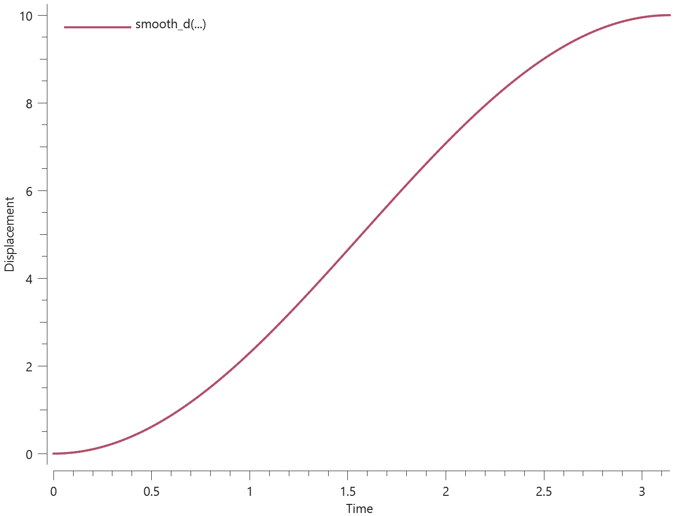
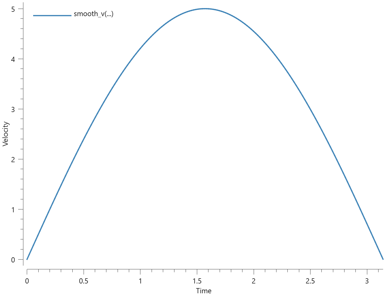
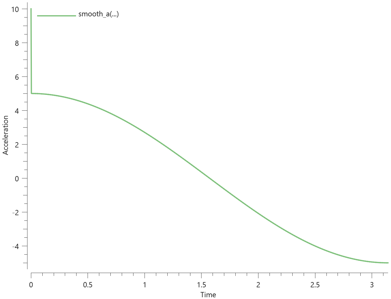
Tests
This benchmark is associated with 1 tests.
*GEOMETRY_BOX
Pressure loading
"Optional title"
gid, csysid
$x_1$, $y_1$, $z_1$, $x_2$, $y_2$, $z_2$
This tests the *GEOMETRY_BOX command. It allows the user to specify a geometry by defining two sets of coordinates. To test the command, *LOAD_PRESSURE is applied in the geometry. A hollow sphere occupies the same geometry, and the momentum of the sphere is checked for version control.
A $0.01 \ MPa$ pressure is applied to a $1x1 \ m$ area of the sphere. The mass of the sphere is a bit less than $1000 \ kg$, and final momentum is checked for version control.
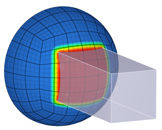
Tests
This benchmark is associated with 1 tests.
*GEOMETRY_COMPOSITE
Bc motion
"Optional title"
gid
gid${}_1$, ..., gid${}_8$
This model tests the functionality of the *GEOMETRY_COMPOSITE command.
Tested parameters: gid, gid${}_1$, gid${}_2$.
Two component boxes are created, see the yellow and grey box in Figure 1. Also two box geometries are created.
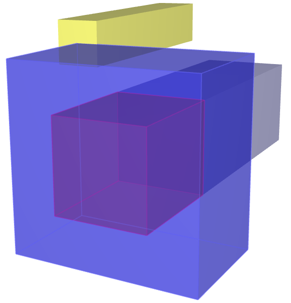
*GEOMETRY_COMPOSITE is being used to remove the smaller box geometry from the larger box geometry. *BC_MOTION is used to prescribe a velocity to the remaining geometry. In this case this means that only the yellow box should move since it has elements that are bordering to the remaining geometry.
Coordinates of both boxes are checked for version control.
Tests
This benchmark is associated with 1 tests.
Load thermal surface
"Optional title"
gid
gid${}_1$, ..., gid${}_8$
Tested parameters: gid, gid${}_1$, gid${}_2$.
This model tests the command *GEOMETRY_COMPOSITE. A square plate is subjected to a thermal surface load. The geometry defining the load pressure is created with *GEOMETRY_COMPOSITE. The composite geometry is created by combining two box geometries of side length $0.8 \ m$ and $0.4 \ m$ respectivly. The smaller box is referenced with a negative ID which removes it from the larger geometry. See Figure 1.
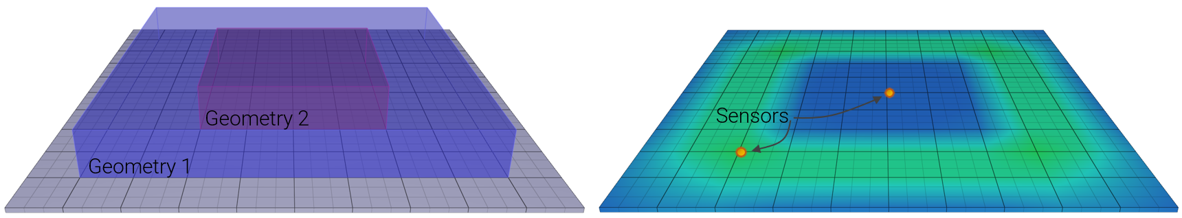
The area of the surface subjected to the thermal load is: $$ A_{Geometry 1} - A_{Geometry 2} = 0.8^2 - 0.4^2 = 0.48 \ m^2 $$
The thermal surface load applied is $1 \ MW/m^2$ giving a total energy supplied to the plate of: $$ 1,000,000 \cdot 0.48 = 480,000 \ J/s $$
The energy supplied from the thermal surface load is presented in Figure 2.
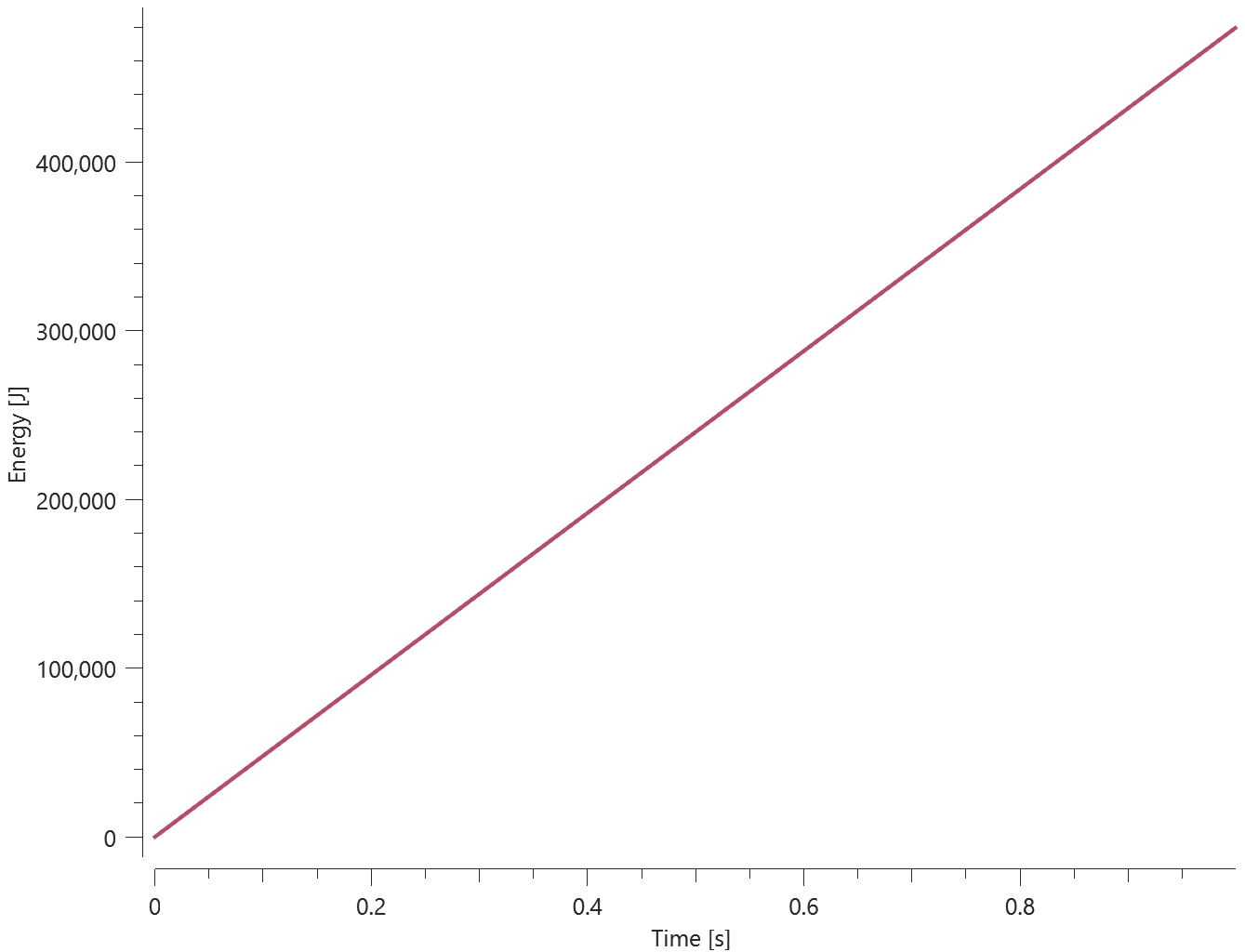
The energy from the thermal surface load and temperature at both sensors are checked for version control.
Tests
This benchmark is associated with 1 tests.
Pressure loading
"Optional title"
gid
gid${}_1$, ..., gid${}_8$
Tested parameters: gid, gid${}_1$, gid${}_2$.
This model tests the command *GEOMETRY_COMPOSITE. A square plate is subjected to a load pressure of $0.01 \ MPa$. The geometry defining the load pressure is created with *GEOMETRY_COMPOSITE. The composite geometry is created by combining two box geometries of side length $0.8 \ m$ and $0.4 \ m$ respectivly. The smaller box is referenced with a negative ID which removes it from the larger geometry. See Figure 1.
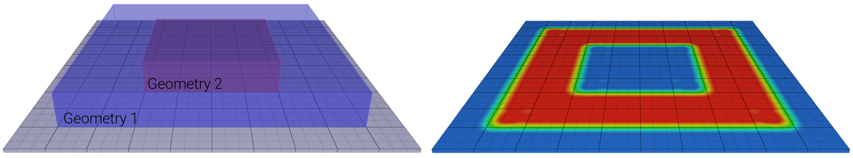
The area of the surface subjected to load pressure is: $$ A_{Geometry 1} - A_{Geometry 2} = 0.8^2 - 0.4^2 = 0.48 \ m^2 $$ The force generated is: $$ F = P \cdot A = 10000 \cdot 0.48 = 4800 \ N $$
The force generated from load_pressure.out is presented in Figure 2.
Tests
This benchmark is associated with 1 tests.
*GEOMETRY_EFP
Particle count
"Optional title"
gid, csysid
$x_1$, $y_1$, $z_1$, $x_2$, $y_2$, $z_2$, $R_1$, $R_2$
$R_3$
Tested parameters: gid, $x_1$, $y_1$, $z_1$, $x_2$, $y_2$, $z_2$, $R_1$, $R_2$, $R_3$.
This model tests the *GEOMETRY_EFP command. An Explosively Formed Projectile is constructed by the use of three geometries generated with *GEOMETRY_EFP. The three geometries will form the Casing, Explosive and Liner volumes that are filled with particles that make up the EFP. This is done with the help of *GEOMETRY_COMPOSITE. Additionaly the wave shaper is created with *GEOMETRY_PIPE.
The test setup is displayed in Figure 1.
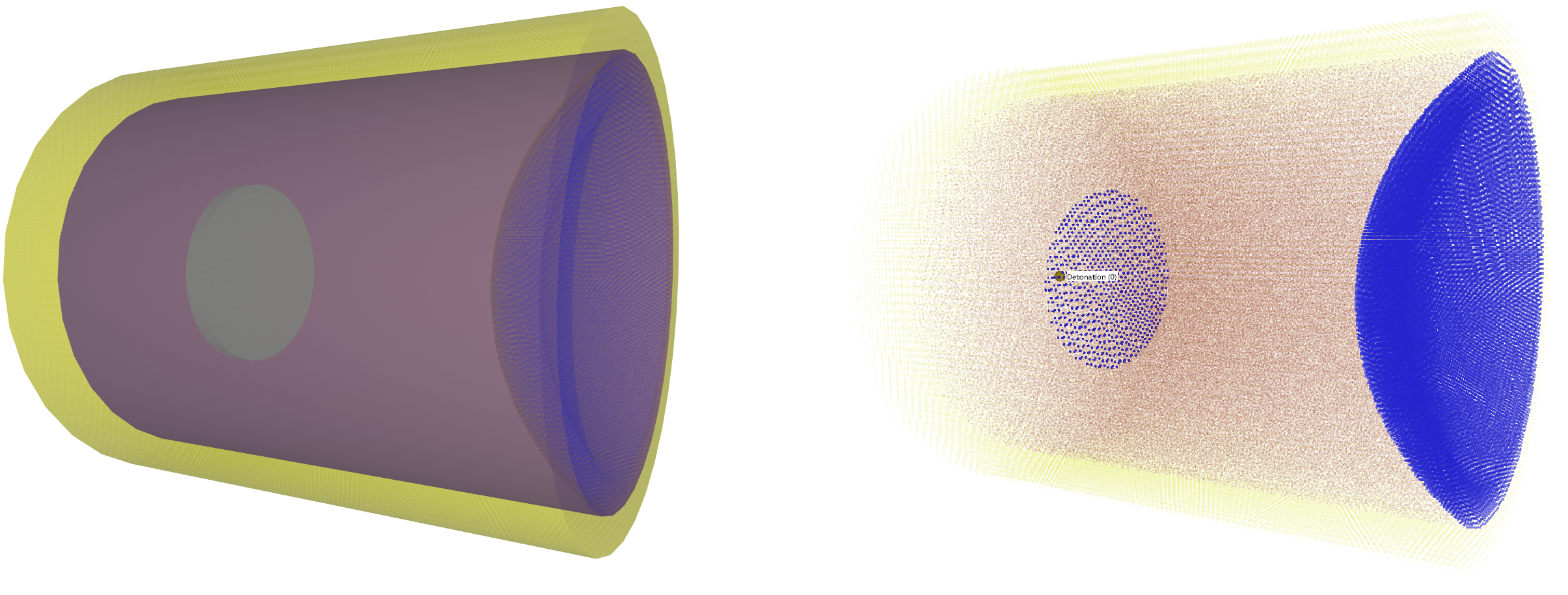
In order to verify that the *GEOMETRY_EFP command is working properly the number of particles of the different geometries at time zero is checked.
The number of particles of the ingoing components of the EFP is presented in Figure 2.

Tests
This benchmark is associated with 1 tests.
*GEOMETRY_PART
Pressure loading
"Optional title"
gid, csysid
pid
This tests the *GEOMETRY_PART command. The model is a simplified version of that found in the *LOAD_PRESSURE benchmark. A pressure is applied to a surface of a structure by a geometry defined from a part. Final momentum of the structure is checked for version control.
Tests
This benchmark is associated with 1 tests.
*GEOMETRY_PIPE
Pressure loading
"Optional title"
gid, csysid
$x_1$, $y_1$, $z_1$, $x_2$, $y_2$, $z_2$, $R_1$, $R_2$
$R_3$, $R_4$, $v_x$, $v_y$, $v_z$, $\alpha$
This tests the *GEOMETRY_PIPE command. It is used to define a straight pipe or cylinder in space by its face center coordinates. To test the command, *LOAD_PRESSURE is applied in the geometry. A hollow sphere occupies the same geometry, and the momentum of the sphere is checked for version control.
Tests
This benchmark is associated with 1 tests.
*GEOMETRY_SEED_COORDINATE
Applied pressure
"Optional title"
gid
$x$, $y$, $z$, $\alpha_c$, pid
This tests the *GEOMETRY_SEED_COORDINATE. The command is used to define a geometry from a coordinate. In this test, a geometry is defined on the surface of a structure and a pressure is applied in the geometry.
Final momentum of the structure is checked for version control.
Tests
This benchmark is associated with 1 tests.
*GEOMETRY_SEED_NODE
Applied pressure
"Optional title"
gid
nid${}_1$, nid${}_2$, $\alpha_c$
This test is similair to the test of *GEOMETRY_SEED_COORDINATE, but in this test, the geometry is created from a seed node with command *GEOMETRY_SEED_NODE. Final momentum of the structure is checked for version control.
Tests
This benchmark is associated with 1 tests.
*GEOMETRY_SPHERE
Load pressure in geometry
"Optional title"
gid, csysid
$x$, $y$, $z$, $R_1$, $R_2$
This tests the *GEOMETRY_SPHERE command. A sphere geometry with radius $4 \ m$ is defined in between two blocks. An pressure of $50 \ kPa$ is applied in the geometry to move the blocks apart. The center of the sphere is at the surface of one of the blocks. The force on this block should therefore be $16 \pi \cdot 50 \ kN$. The other block is at a distance of $2 \ m$ from the center of the sphere. Expected force on this block is $12\pi \cdot 50 \ kN$. These targets are used for version control by checking the final momentums of both blocks.
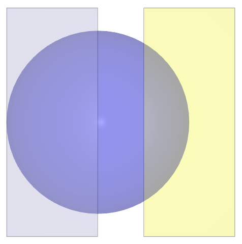
Tests
This benchmark is associated with 1 tests.
*INCLUDE
Offset
"Optional title"
filename
$sf_x$, $sf_y$, $sf_z$, nid_offset, eid_offset, pid_offset, mid_offset, gid_offset
$x_0$, $y_0$, $z_0$, $x_1$, $y_1$, $z_1$
$\bar{x}_{x}$, $\bar{x}_{y}$, $\bar{x}_{z}$, $\bar{y}_{x}$, $\bar{y}_{y}$, $\bar{y}_{z}$, mirror
Tested parameters: nid_offset, eid_offset, pid_offset, mid_offset, gid_offset.
This model tests the offset parameters in the *INCLUDE command. In total three files are used, "main.k", "sub.k" and "element_offset.k". In the "main.k" file the file "sub.k" is included with an offset of 100, 200, 990, 995, 999 to nid_offset, eid_offset, pid_offset, mid_offset, gid_offset respectively.
To see that gid_offset works properly, functions are created within "sub.k" that returns the Y- and Z-coordinates of a sensor that is created in "main.k". The sensor ID should thus be 999+sensor ID.
In "sub.k, "element_offset.k" is included which defines a cube from 8 solid element. To see that mid_offset and pid_offset is working properly the material ID and part ID in the "main.k" file should be 995+material ID, 990+Part ID. Also the element ID's and Node ID's should be 200+Element ID and 100+Node ID. This is checked with Output node and Output element.
Targets:
- First cube should rotate 1 lap about X-axis
- Second cube should move downwards 1 m in Z-direction
Tests
This benchmark is associated with 1 tests.
Test 1
"Optional title"
filename
$sf_x$, $sf_y$, $sf_z$, nid_offset, eid_offset, pid_offset, mid_offset, gid_offset
$x_0$, $y_0$, $z_0$, $x_1$, $y_1$, $z_1$
$\bar{x}_{x}$, $\bar{x}_{y}$, $\bar{x}_{z}$, $\bar{y}_{x}$, $\bar{y}_{y}$, $\bar{y}_{z}$, mirror
This tests the *INCLUDE command. A mesh file is included, then transformed and scaled. The model is a single cubic element. Coordinates of two oppsite corners are checked in "node.out" for version control.
Tests
This benchmark is associated with 1 tests.
*INCLUDE_BINARY
Binary elements
filename
In this benchmark all avalible element types are imported as a binary mesh. The physical mass of each element are checked for version control.
Tests
This benchmark is associated with 1 tests.
Binary mesh
filename
Tested functionality:
Importing a binary mesh and running a simulation.
A binary mesh of two long rods is imported using *INCLUDE_BINARY. A simulation is then run, and the mass of the parts are then checked for verison control.
Simulation continued from .bin
filename
Tested functionality:
Import results from one simulation and use it to define the initial state in another model.
If running the model in one step the Z-coordinate of the back face is $Z=6.654e^{-3}$ at time $t=10 \ \mu s$. The simulation is split into two steps, the first from $t=0$ to $t=2 \ \mu s$ and the second from $t=2 \ \mu s$ to $t=10 \ \mu s$.
Step 1 ($0 - 2 \ \mu s$): Has already been completed and the state is stored in impetus_state1.k and impetus_state1.bin.
Step 2 ($2 - 10 \ \mu s$): Current model.
Target:
If the end result from Step 1 is correctly imported to Step 2, the back face should be at $Z=6.654e^{-3}$ at termination.
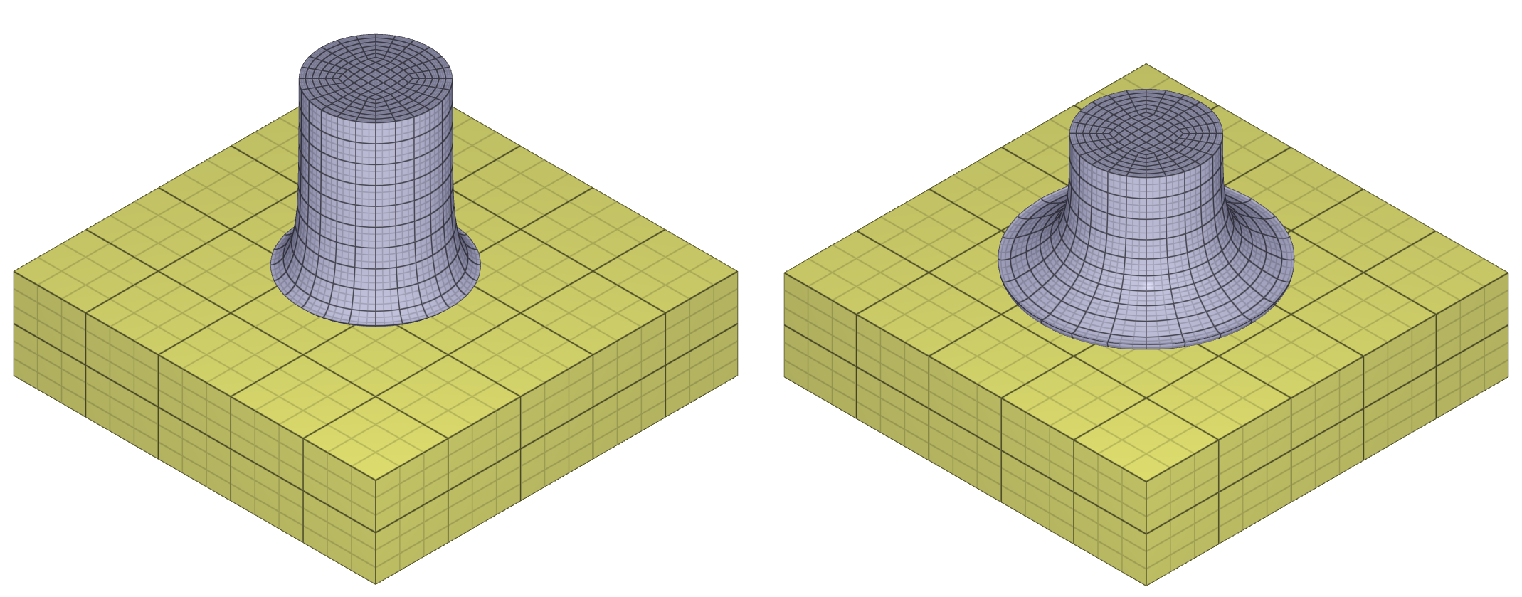
Tests
This benchmark is associated with 3 tests.
*INITIAL_DAMAGE_RANDOM
Cubes with random initial damage
entype, enid, $a$, $b$, $D_{max}$, $R$, cid, did
Randomly distributed initial damage is defined on a model consisting of $32 \times 32$ geometrically identical cubes, as presented in Figure 1. The number of cubes is assumed to be enough to consider the test valid from a statistical point of view. Each cube is constructed by a single linear hexahedral element.
The initial damage in each element is uniform throughout the entire element which is achieved by utilizing an imperfection radii (a built-in parameter in *INITIAL_DAMAGE_RANDOM).
A prescribed velocity is imposed at one of the cubes surfaces while the opposite surface of the cubes is fixed in the direction of the prescribed velocity, hence the cubes are uni-axially stretched. The plastic work that has been accomplished when the final cube/element is eroded due to fully developed damage is checked against the same quantity obtained from an alternative numerical approach.
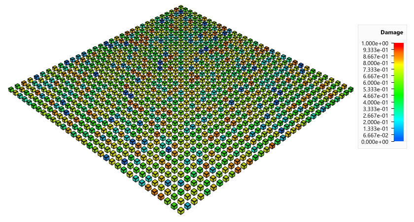
Tests
This benchmark is associated with 1 tests.
Distribution in integration points
entype, enid, $a$, $b$, $D_{max}$, $R$, cid, did
In this test the damage distribution from *INITIAL_DAMAGE_RANDOM is tested. A cubic part with 1000 LHEX elements is subjet for initial damage. The damage is randomly distributed in each elements 8 integration points. The data from the elements is then extracted and compared with an analytical result.
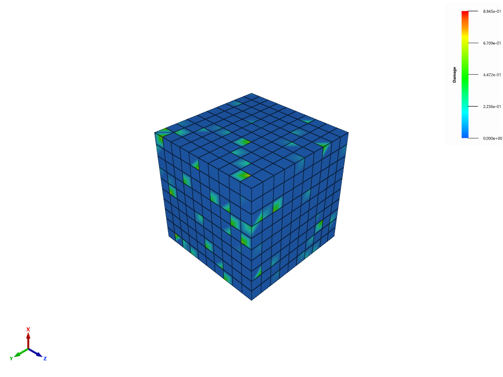
The first, last and average value of the initial damage curve are checked against the analytical target curve.
Tests
This benchmark is associated with 1 tests.
Function to describe defect distribution
entype, enid, $a$, $b$, $D_{max}$, $R$, cid, did
Randomly distributed initial damage is defined on a model consisting of $100 \times 100$ geometrically identical cubes, as presented in Figure 1.
To ensure randomness, a new damage distribution is generated each time the solver starts with the command *RANDOM_NUMBER_GENERATOR_SEED. The number of cubes is assumed to be enough to consider the test valid from a statistical point of view. Each cube is constructed by a single linear hexahedral element.
The initial damage in each element is uniform throughout the entire element which is achieved by utilizing an imperfection radii (a built-in parameter in *INITIAL_DAMAGE_RANDOM).
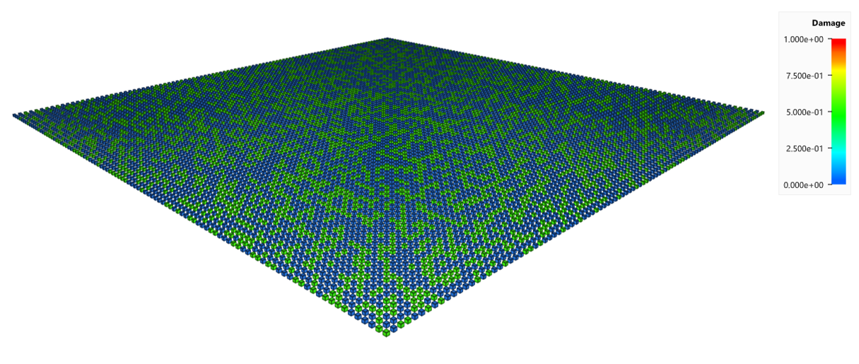
The randomly distributed initial damage is defined to the model by assigning a Heaviside step function to the distribution function $f(D)$, which describes the number of defects $N$ per unit volume of matter. The initial damage is only allowed to be within the range of $0.49-0.51$. The probability $p$ that an element is assigned an initial damage is:
$$ p = 1-e^{-N \cdot v} $$
Where $v$ is the element volume and $N$ the number of defects per unit volume. With $N=500$ and $v=0.001$, $p$ is:
$$ p = 1-e^{-500 \cdot 0.001} = 0.39347 $$
The elements are uni-axially stretched to the point to which only the elements with an initial damage are eroded. The final volume of the model is then:
$$ V_{final} = V_{initial} \cdot (1-p) $$
Where $V_{final}$ is the final volume and $V_{initial}$ the initial volume of the model. With $V_{initial} =10$ The final volume should be:
$$ V_{final} = 10 \cdot (1-0.39347) = 6.0653 $$
This can be seen by tracking the total volume of the model. Volume vs. time can be seen in Figure 2.
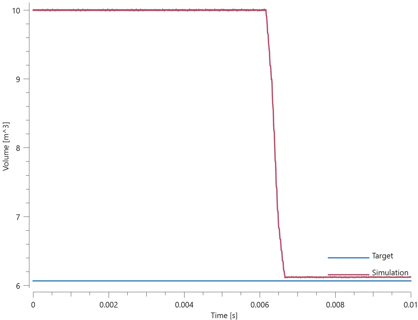
First and last value of volume is checked for version control.
Tests
This benchmark is associated with 1 tests.
*INITIAL_DAMAGE_SURFACE_RANDOM
Surface with random initial damage
entype, enid, $\Delta_0$, $m$, $D_{max}$, $R$, cid
Tested parameters: entype, enid, $\Delta_0$, $m$, $D_{max}$, $R$.
The model tests the *INITIAL_DAMAGE_SURFACE_RANDOM command.
Randomly distributed initial damage is defined on the top surface of a plate consisting of $32 \times 32$ linear hexahedral element, as presented in Figure 1. The number of elements is assumed to be enough to consider the test valid from a statistical point of view.
A prescribed velocity is imposed at the top surface of the model while the opposite surface is fixed in the direction of the prescribed velocity, hence the model is uni-axially stretched. Failed elments are eroded. The plastic work that has been accomplished when the final element is eroded due to fully developed damage is checked against the same quantity obtained from an alternative numerical approach.
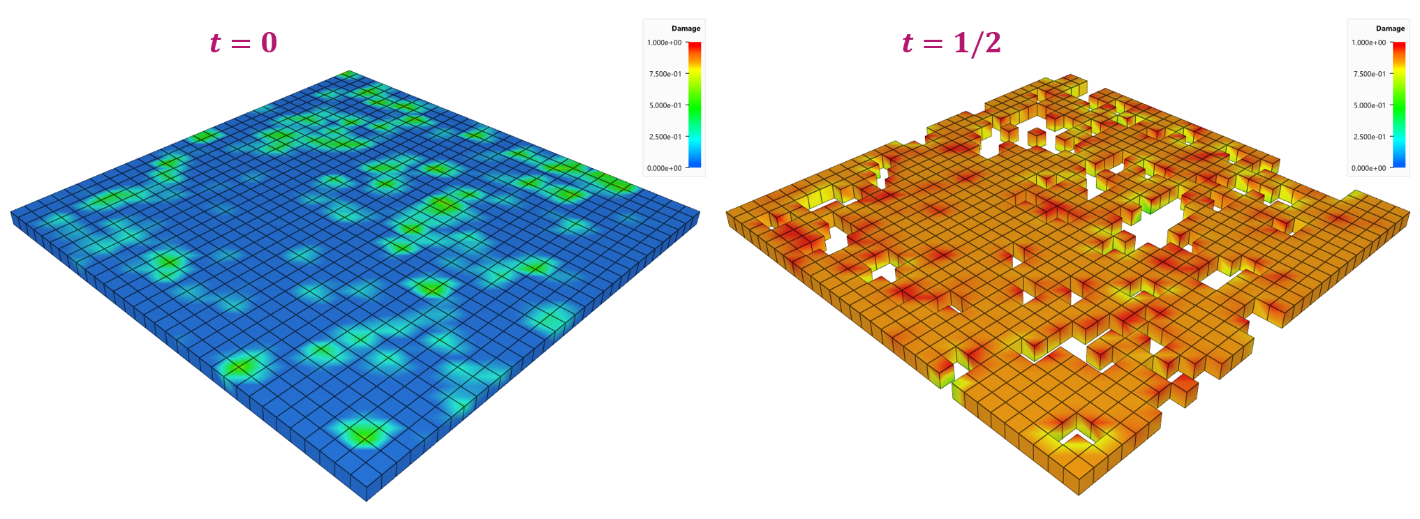
Tests
This benchmark is associated with 1 tests.
*INITIAL_DISPLACEMENT
Reposition nodes
"Optional title"
entype, enid, $d_{x}$, $d_{y}$, $d_{z}$
This model tests the command *INITIAL_DISPLACEMENT. The nodes of an element is repositioned at time zero.
The x-coordinate center of gravity of the part should go from $0 \ to \ 1$. The test is checked for version control.
Tests
This benchmark is associated with 1 tests.
*INITIAL_MATERIAL_DIRECTION
Test 1
"Optional title"
nid, $\hat{x}_x$, $\hat{x}_y$, $\hat{x}_z$, $\bar{y}_x$, $\bar{y}_y$, $\bar{y}_z$
The command *INITIAL_MATERIAL_DIRECTION is used to define material directions in anisotropic materials. In this command the material direction is defined by use of the element corner nodes.
The test consists of three hexahedron elements, one of each type (linear/quadratic/cubic). Each element is assigned a unique material direction. The fiber direction is defined in the X-direction for the linear element, in the Y-direction for the quadratic element and in the Z-direction for the cubic element.
The elements are then stretched, first in the X-direction, then in the Y-direction and lastly in the Z-direction. The elements restore the original geometry between the stretches and therefore the loading is uniaxial.
The material used have a stiffness of $10 \ GPa$ in the fiber direction and $5 \ GPa$ perpendicular to the fibers. The maximum stretch in each direction is 5% (nominal).
The maximum stress in the fiber direction should therefore be $10e9 \cdot ln(1+0.05) \approx 487.9 \ MPa$ and $5e9 \cdot ln(1+0.05) \approx 244.0 \ MPa$ perpendicular to the fiber direction. This is checked in the version control.
Figure 1 shows the results from the latest version control together with targets.

Tests
This benchmark is associated with 1 tests.
*INITIAL_MATERIAL_DIRECTION_PATH
Material fiber direction split
"Optional title"
coid, entype, enid, pathid
Tested parameters: coid, entype, enid, pathid.
This model tests functionality of the command *INITIAL_MATERIAL_DIRECTION_PATH. The model tests that material fiber directions are interpolated between paths that are split into two segments. For reference two components are used, one with the fiber directions along a single path and the other one with fiber directions interpolated between two paths. See Figure 1
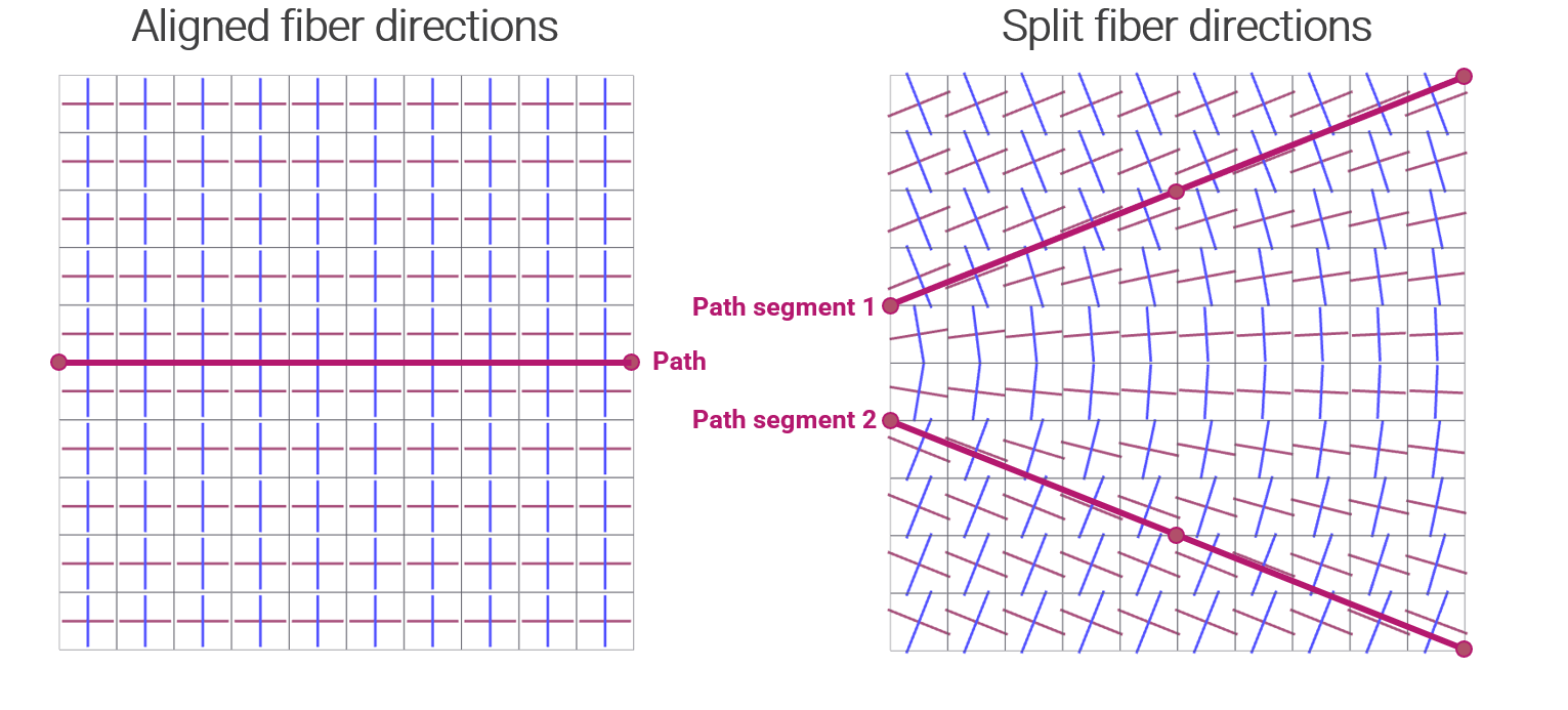
Both components are modelled with one element in the thickness direction. One side of the components is fixed and the other side is given a prescribed velocity in the X-direction. To distinguish the effect that fiber direction has, output sensors are placed at given locations to measure displacements. Figure 2
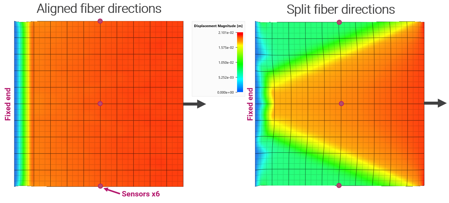
Maximum X-displacements at the sensors are checked for version control.
Tests
This benchmark is associated with 1 tests.
Material fiber direction split (multiple elements in thickness direction)
"Optional title"
coid, entype, enid, pathid
The model tests initial material directions when using multiple elements in the thickness direction. This test is similar to the test "*INITIAL_MATERIAL_DIRECTION_PATH - Material fiber direction split".
Tests
This benchmark is associated with 1 tests.
Test 1
"Optional title"
coid, entype, enid, pathid
The command *INITIAL_MATERIAL_DIRECTION_PATH is used to define material directions in anisotropic materials. In this command the material direction is defined by user defined paths.
The test consists of three hexahedron elements, one of each type (linear/quadratic/cubic). Each element is assigned a unique material direction. The fiber direction is defined in the X-direction for the linear element, in the Y-direction for the quadratic element and in the Z-direction for the cubic element.
The elements are then stretched, first in the X-direction, then in the Y-direction and lastly in the Z-direction. The elements restore the original geometry between the stretches and therefore the loading is uniaxial.
The material used have a stiffness of $10 \ GPa$ in the fiber direction and $5 \ GPa$ perpendicular to the fibers. The maximum stretch in each direction is 5% (nominal).
The maximum stress in the fiber direction should therefore be $10e9 \cdot ln(1+0.05) \approx 487.9 \ MPa$ and $5e9 \cdot ln(1+0.05) \approx 244.0 \ MPa$ perpendicular to the fiber direction. This is checked in the version control.
Figure 1 shows the results from the latest version control together with targets.

Tests
This benchmark is associated with 1 tests.
*INITIAL_MATERIAL_DIRECTION_VECTOR
Surface normal determination
"Optional title"
coid, entype, enid
$\hat{x}_x$, $\hat{x}_y$, $\hat{x}_z$, $\bar{y}_x$, $\bar{y}_y$, $\bar{y}_z$
This model tests the automatic determination of the face normals of a pipe geometry with the command *INITIAL_MATERIAL_DIRECTION_VECTOR.
The direction of the local x-axis is specified to be (1,0,0) which is the central axis of the pipe. The local y-axis is determined from the cross product of the local z- and x-axis.
$$\hat{y} = \hat{z} \ X \ \hat{x}$$
Where the local z-axis is equivalent to the local element face normal $\hat{z} = \hat{n}$ which is automatically determined by the solver.
The test setup is displayed in Figure 1.
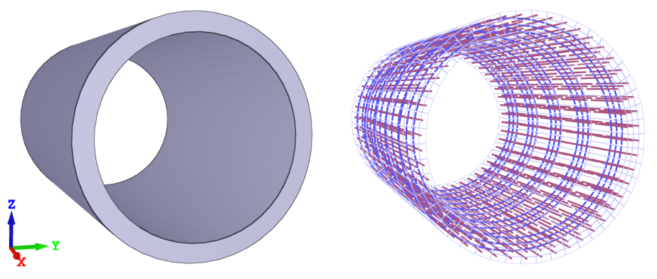
An internal pressure is added to the model. The radius of the pipe should expand uniformally. See Figure 2.
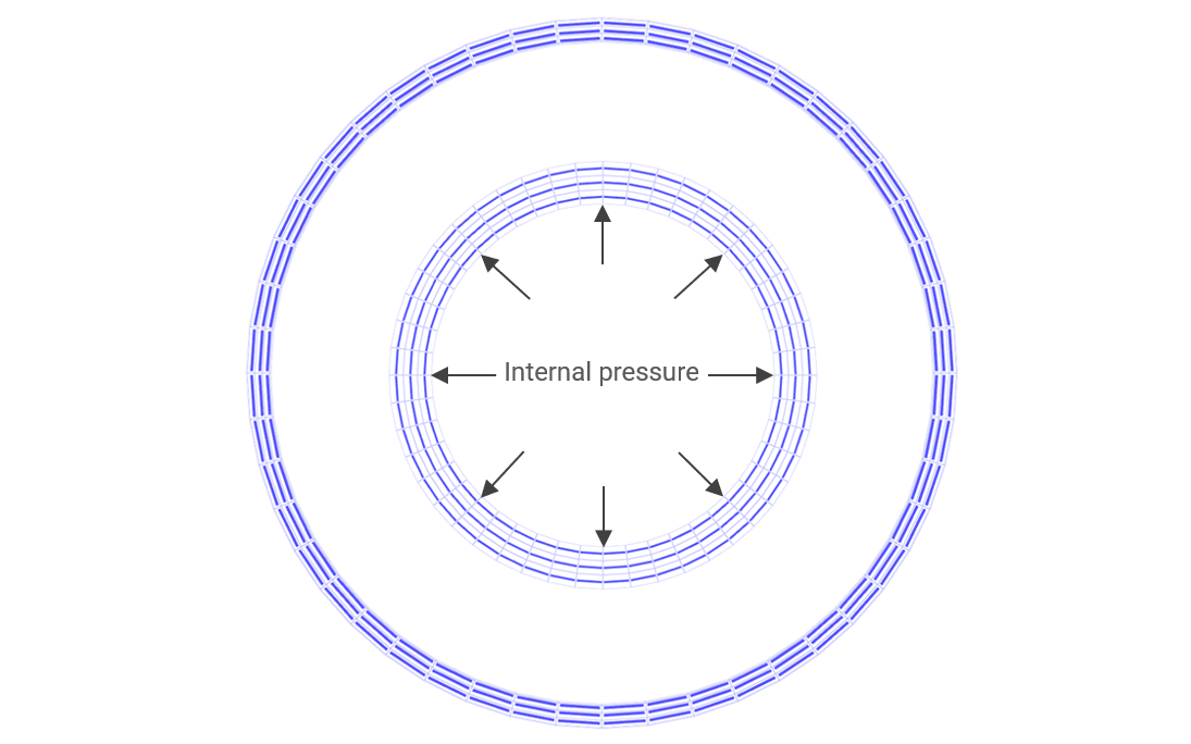
Tests
This benchmark is associated with 1 tests.
Test 1
"Optional title"
coid, entype, enid
$\hat{x}_x$, $\hat{x}_y$, $\hat{x}_z$, $\bar{y}_x$, $\bar{y}_y$, $\bar{y}_z$
The command *INITIAL_MATERIAL_DIRECTION_VECTOR is used to define material directions in anisotropic materials. In this command the material direction is defined by user defined vectors.
The test consists of three hexahedron elements, one of each type (linear/quadratic/cubic). Each element is assigned a unique material direction. The fiber direction is defined in the X-direction for the linear element, in the Y-direction for the quadratic element and in the Z-direction for the cubic element.
The elements are then stretched, first in the X-direction, then in the Y-direction and lastly in the Z-direction. The elements restore the original geometry between the stretches and therefore the loading is uniaxial.
The material used have a stiffness of $10 \ GPa$ in the fiber direction and $5 \ GPa$ perpendicular to the fibers. The maximum stretch in each direction is 5% (nominal).
The maximum stress in the fiber direction should therefore be $10e9 \cdot ln(1+0.05) \approx 487.9 \ MPa$ and $5e9 \cdot ln(1+0.05) \approx 244.0 \ MPa$ perpendicular to the fiber direction. This is checked in the version control.
Figure 1 shows the results from the latest version control together with targets.

Tests
This benchmark is associated with 1 tests.
*INITIAL_MATERIAL_DIRECTION_WRAP
Test 1
"Optional title"
coid, entype, enid
$x_0$, $y_0$, $z_0$, $\hat{u}_x$, $\hat{u}_y$, $\hat{u}_z$, $\alpha$
The command *INITIAL_MATERIAL_DIRECTION_WRAP is used to define material directions in anisotropic materials. In this command the material direction is defined by a user defined "ply" in space that is wrapped around the component.
The test consists of three hexahedron elements, one of each type (linear/quadratic/cubic). Each element is assigned a unique material direction. The fiber direction is defined in the X-direction for the linear element, in the Y-direction for the quadratic element and in the Z-direction for the cubic element.
The elements are then stretched, first in the X-direction, then in the Y-direction and lastly in the Z-direction. The elements restore the original geometry between the stretches and therefore the loading is uniaxial.
The material used have a stiffness of $10 \ GPa$ in the fiber direction and $5 \ GPa$ perpendicular to the fibers. The maximum stretch in each direction is 5% (nominal).
The maximum stress in the fiber direction should therefore be $10e9 \cdot ln(1+0.05) \approx 487.9 \ MPa$ and $5e9 \cdot ln(1+0.05) \approx 244.0 \ MPa$ perpendicular to the fiber direction. This is checked in the version control.
Figure 1 shows the results from the latest version control together with targets.
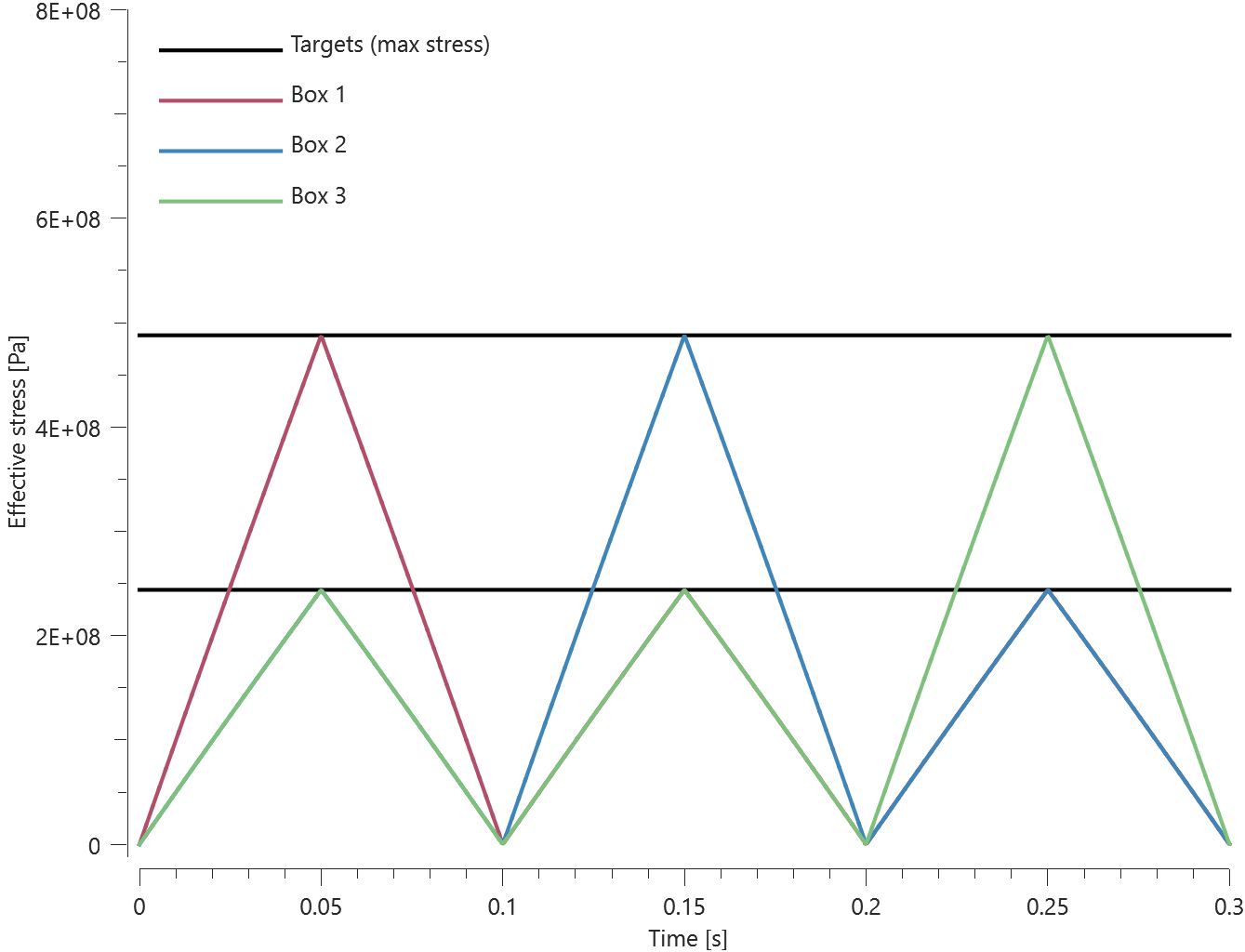
Tests
This benchmark is associated with 1 tests.
*INITIAL_PLASTIC_STRAIN_FUNCTION
Multiple initial plastic strains
coid, entype, enid, fid, multi
Tested parameters: coid, entype, enid, fid, multi.
The model tests the command *INITIAL_PLASTIC_STRAIN_FUNCTION. The command is used to prescribe initial plastic strains. Two options are available when implementing the initial plastic strains:
- Option 1 (multi = 0): plastic strains from previous commands are overwritten
- Option 2 (multi = 1): plastic strains from multiple commands are superimposed
To test both options, two bars with identical dimensions are given an initial plastic strain in two steps:
-First step, the bars are given an initial plastic strain linearly distributed from 0 at one end to 0.05 at the other end.
-Second step, the bars are given an initial plastic strain of 0.10 with option 1 for bar 1 and option 2 for bar 2.
This means that the maximum initial plastic strain in aggregate should be 0.1 for bar 1 and 0.15 for bar 2.
See Figure 1.
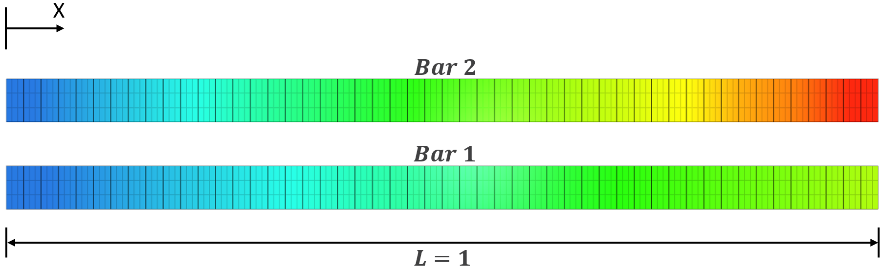
Output sensors are placed at the middle and at the end of the beams to measure effective plastic strains.
The first values of effective plastic strain is checked for version control.
Tests
This benchmark is associated with 1 tests.
*INITIAL_STATE_HAZ
Strain in HAZ model
entype${}_{weld}$, enid${}_{weld}$, entype${}_{base}$, enid${}_{base}$, cid${}_{sigy}$, cid${}_{D0}$
This tests the command *INITIAL_STATE_HAZ. It is used to define mechanical properties in a heat affected zone (HAZ) after a welding operation. Initial yield stress and damage are defined as functions of the distance from the weld. In the test model, two plates have been welded to a beam. The plates are pulled apart. Maximum reaction force is checked for version control.
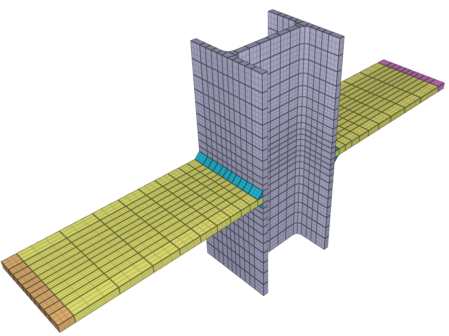
Tests
This benchmark is associated with 1 tests.
*INITIAL_STRESS_FUNCTION
Test 1
entype, enid, fid${}_{xx}$, fid${}_{yy}$, fid${}_{zz}$, fid${}_{xy}$, fid${}_{yz}$, fid${}_{zx}$
multi
An initial stress state can be included by the command *INITIAL_STRESS_FUNCTION. Three different options are available when implementing the initial stress state:
- Option 1 (multi = 0): stresses from previous commands are overwritten
- Option 2 (multi = 1): stresses from multiple commands are superimposed
- Option 3 (multi = 2): stress component with largest absolute value is kept
Three identical plates are used in the verification of this command. Each plate have a sensor in the center to extract the stress state in the plate.
First, a stress state (in MPa) according to $\bar{\sigma}_{state,1}$ is imposed on all three plates with option 1.
$$ \bar{\sigma}_{state,1} = \bar{\sigma}_{plate,1} = \begin{bmatrix} 100 & 10 & 20 \\ 10 & 150 & 15 \\ 20 & 15 & 200 \end{bmatrix} $$
The stresses in sensor.out for the first plate is checked in sensor.out.
Another stress state $\bar{\sigma}_{state,2}$ is then imposed on the second and the third plate, with option 2 in the second plate and option 3 in the third plate.
$$ \bar{\sigma}_{state,2} = \begin{bmatrix} -200 & 20 & 40 \\ 20 & -300 & 30 \\ 40 & 30 & -400 \end{bmatrix} $$
The state of stress in the second and the third plate should be in accordance to $\bar{\sigma}{plate,2}$ and $\bar{\sigma}{plate,3}$.
$$ \bar{\sigma}_{plate,2} = \begin{bmatrix} -100 & 30 & 60 \\ 30 & -150 & 45 \\ 60 & 45 & -200 \end{bmatrix} $$
$$ \bar{\sigma}_{plate,3} = \begin{bmatrix} -200 & 20 & 40 \\ 20 & -300 & 30 \\ 40 & 30 & -400 \end{bmatrix} $$
Tests
This benchmark is associated with 1 tests.
*INITIAL_TEMPERATURE
SPH and FE parts
entype, enid, fid, $T$
This test verifies that inital temperatures defined with entype = ALL operates as expected. An initial temperatures are imposed on four different parts. Two of the parts are defined with SPH and two with FE. The temperature of each part at initiation and termination is checked.
Testet parameters: entype, $T$.
The last value of the temperature is check in each part.
Tests
This benchmark is associated with 1 tests.
SPH parts
entype, enid, fid, $T$
This test verifies that inital temperatures defined with entype = sph operates as expected. Four different initial temperatures are imposed on four different SPH parts. The temperature of each part at initiation and termination is checked.
Testet parameters: entype, $T$.
Last values of the tempereature is checked for all parts.
Tests
This benchmark is associated with 1 tests.
Thermal plates
entype, enid, fid, $T$
This model tests the command *INITIAL_TEMPERATURE. Three adjacent blocks are given an INITIAL_TEMPERATURE of $-50 \ K$, $50 \ K$ and $150 \ K$. The outer blocks are moving in slightly towards the inner block so that they intersect. No contact is defined. With sensors located at the intersection between the blocks, it is checked that the temperature are still the same.
Tests
This benchmark is associated with 1 tests.
*INITIAL_THICKNESS
Multi-step forming
nid, thickness
Tested parameters: nid, thickness.
The command *INITIAL_THICKNESS is tested in a simple multi-step forming operation test. The test consists of 2 steps. A single cubic hex element is stretched 2 times in the X-direction reducing its thickness. To keep track of the sheet thickness reduction, the command *OUTPUT_FORMING is used to activate the calculation and output of sheet thickness. This is done through node based initial component thickness (*INITIAL_THICKNESS) which is automatically generated by the Solver Engine when writing a state file. The test setup is seen in Figure 1.
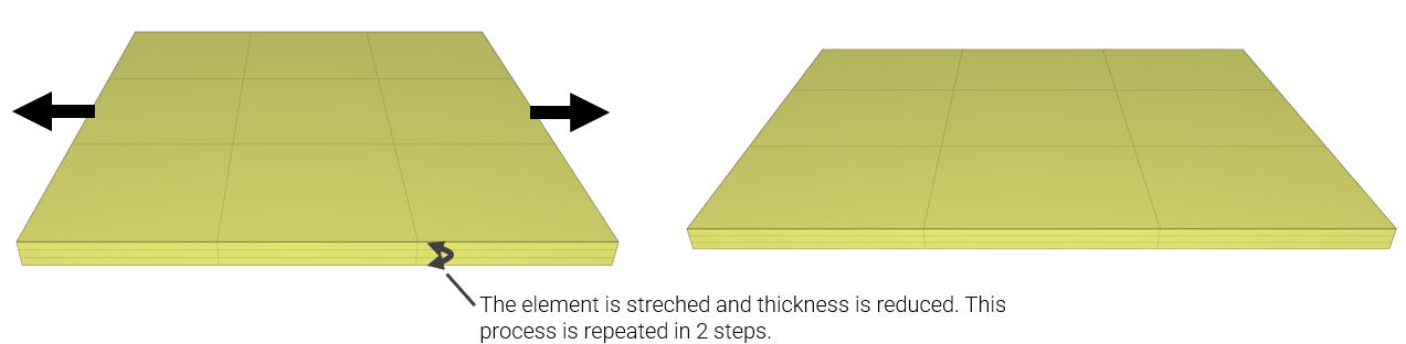
In step 1, the thickness is reduced from $10$ to $9.54 \ mm.$
In step 2, the output from step 1 is included and the element is further streched. The ingoing thickness of $9.54$ is reduced to $9.13 \ mm.$ With an initial thickness of $10 \ mm$ in step 1, the total thickness reduction should be 8.7%.
Final thickness and thickness reduction is checked for version control.
Tests
This benchmark is associated with 2 tests.
*INITIAL_VELOCITY
Cubic element
entype, enid, $v_{x0}$, $v_{y0}$, $v_{z0}$, $\omega_x$, $\omega_y$, $\omega_z$
$x_0$, $y_0$, $z_0$, $\delta v_x$, $\delta v_y$, $\delta v_z$, csysid
This tests the *INITIAL_VELOCITY command. A single cubic element created with *COMPONENT_BOX is given an initial velocity of $5 \ m/s$ in the positive Z-direction. *LOAD_GRAVITY act along the same axis and brings the element to halt before returning to its starting point after $1 \ s$. Initial velocity is checked against "rigid.out" and maximum displacement (target: $1.25 \ m$) is checked against "node.out".
Tests
This benchmark is associated with 1 tests.
*LOAD_AIR_BLAST
Diffraction
"Optional title"
coid
entype, enid, $mtnt$, $x_c$, $y_c$, $z_c$, tid, diffract
toff, ground, $t_{end}$
Three boxes (*COMPONENT_BOX) and three charges (*LOAD_AIR_BLAST) are positioned as displayed in Figure 1, in which the charges are illustrated with spheres. The charges are of the same size and should only affect the box closest to the charge. Different diffraction levels are used for each box: = 0 for box 1, = 1 for box 2 and = 2 for box 3.
The surface pressure is measured at three different locations on each box: the outer surface (surface closest to the charge), the top surface and the inner surface. This is done by using sensors (*OUTPUT_SENSOR).
The pressure at the outer surface should be equal for all boxes. At the top surface, the pressure should be zero for box 1 and non-zero for box 2 and 3. At the inner surface, the pressure should be zero for box 1 and 2 and non-zero for box 3. The pressure at each surface is plotted vs. time in Figure 2 - 4.
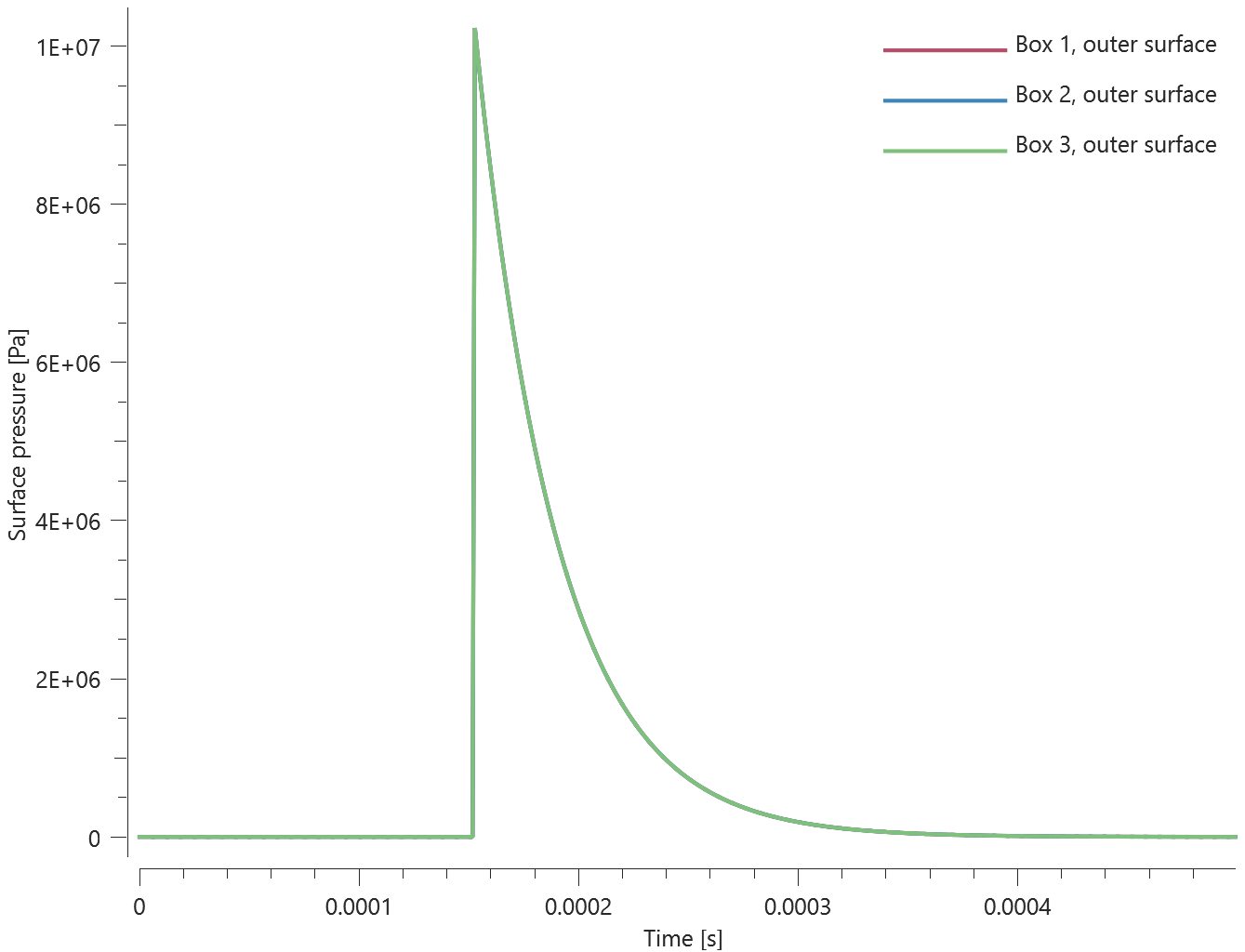
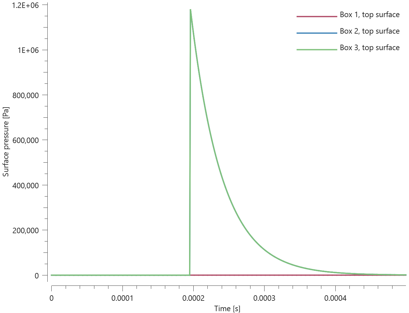
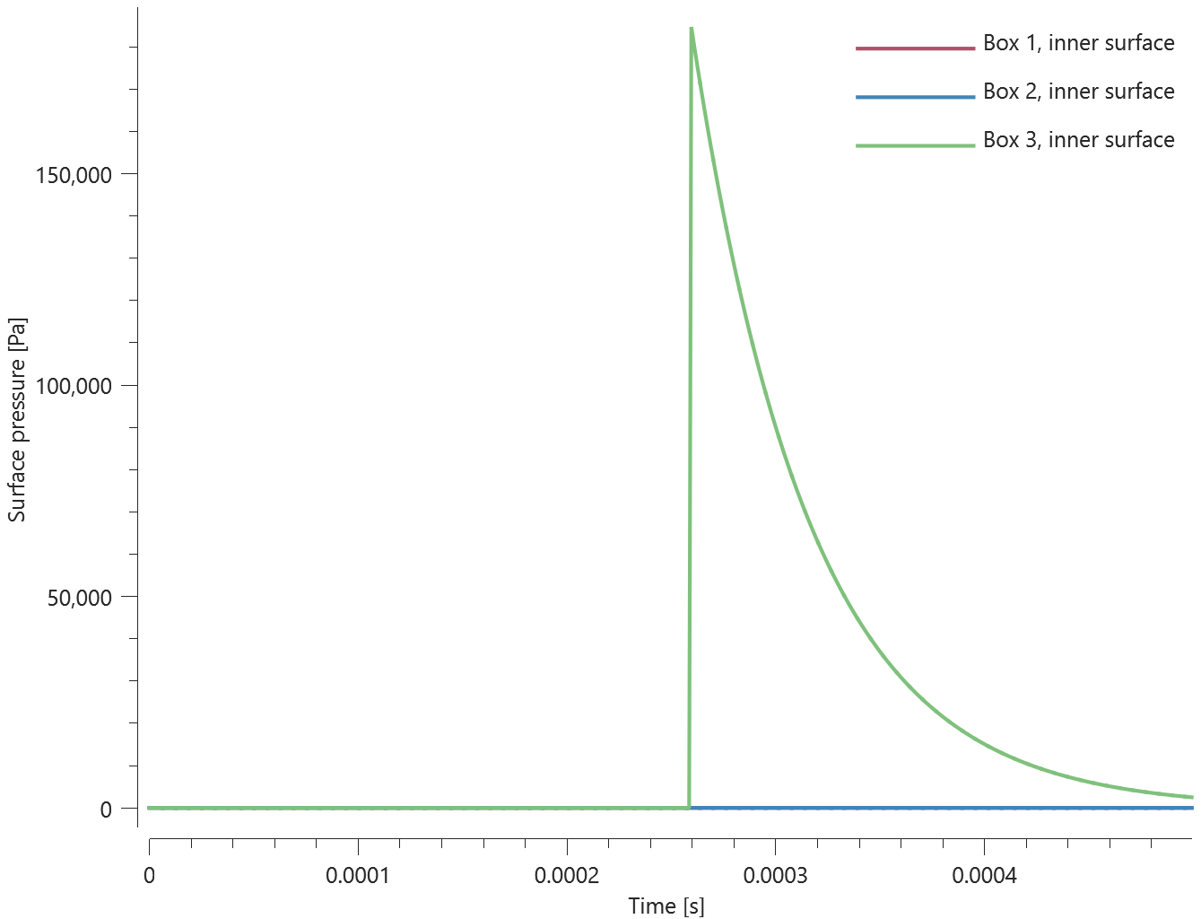
Tests
This benchmark is associated with 1 tests.
Incident pressure
"Optional title"
coid
entype, enid, $mtnt$, $x_c$, $y_c$, $z_c$, tid, diffract
toff, ground, $t_{end}$
The model consists of a spherical explosive charge and a slender structure with a quadratic cross-section (L >> H, W = H). The structure is aligned to the charge in such a way that the blast wave propagates along the length of the structure, parallel to one of the structures faces. The side-on pressure on this face is measured using sensors (*OUTPUT_SENSOR) located at different distances from the charge. An illustration of the test model is presented in Figure 1.
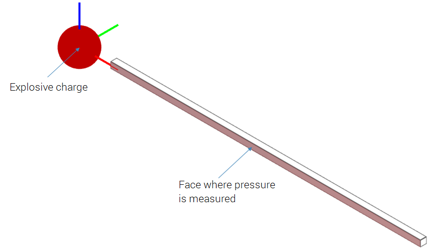
The peak incident pressure at eight different scaled distances in the range of $0.5 - 10$ is compared to emperical data from M. Swisdak, Jr, (1994) [1]. The comparison is displayed in Figure 2 and 3.
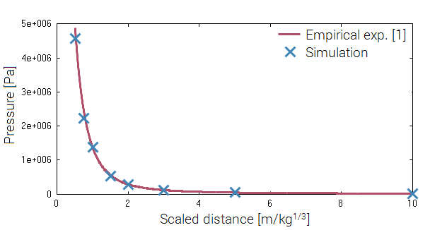
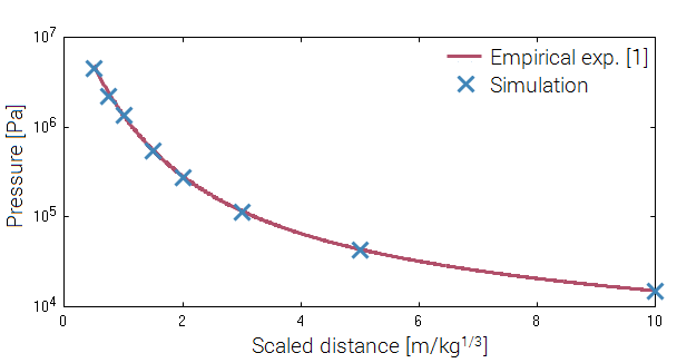
Reference
[1] - Swisdak M. (1994), Simplified Kingery Airblast Calculations, Naval Surface Warfare Center.
Tests
This benchmark is associated with 1 tests.
Reflection
"Optional title"
coid
entype, enid, $mtnt$, $x_c$, $y_c$, $z_c$, tid, diffract
toff, ground, $t_{end}$
The model consists of four quadratic plates and two explosive charges, positioned as displayed in Figure 1. Two charges are included by using two *LOAD_AIR_BLAST-commands.
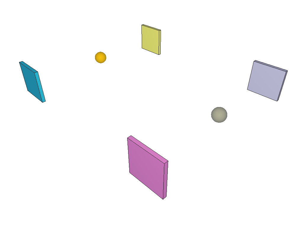
Plate 1 and 2 are located on opposite sides of one of the charges. These plates are included in a part set. One of the charges are defined to impinge this part set and reflectivity is assumed. The other charge is defined to affect plate 3 without any reflectivity. Plate 4 is not affected by any of the charges.
For both air blasts, the time offset flag is set to 1, meaning that the time of arrival of the pressure pulse is defined as time = 0.
The max peak pressure for plate 1, 2 and 3 should be equal while the pressure in plate 4 should be zero at all time. For plate 1 and 2, an additional pressure pulse should be seen after the initial pressure pulse due to the reflectivity. The pressure vs. time for the plates are presented in Figure 2.
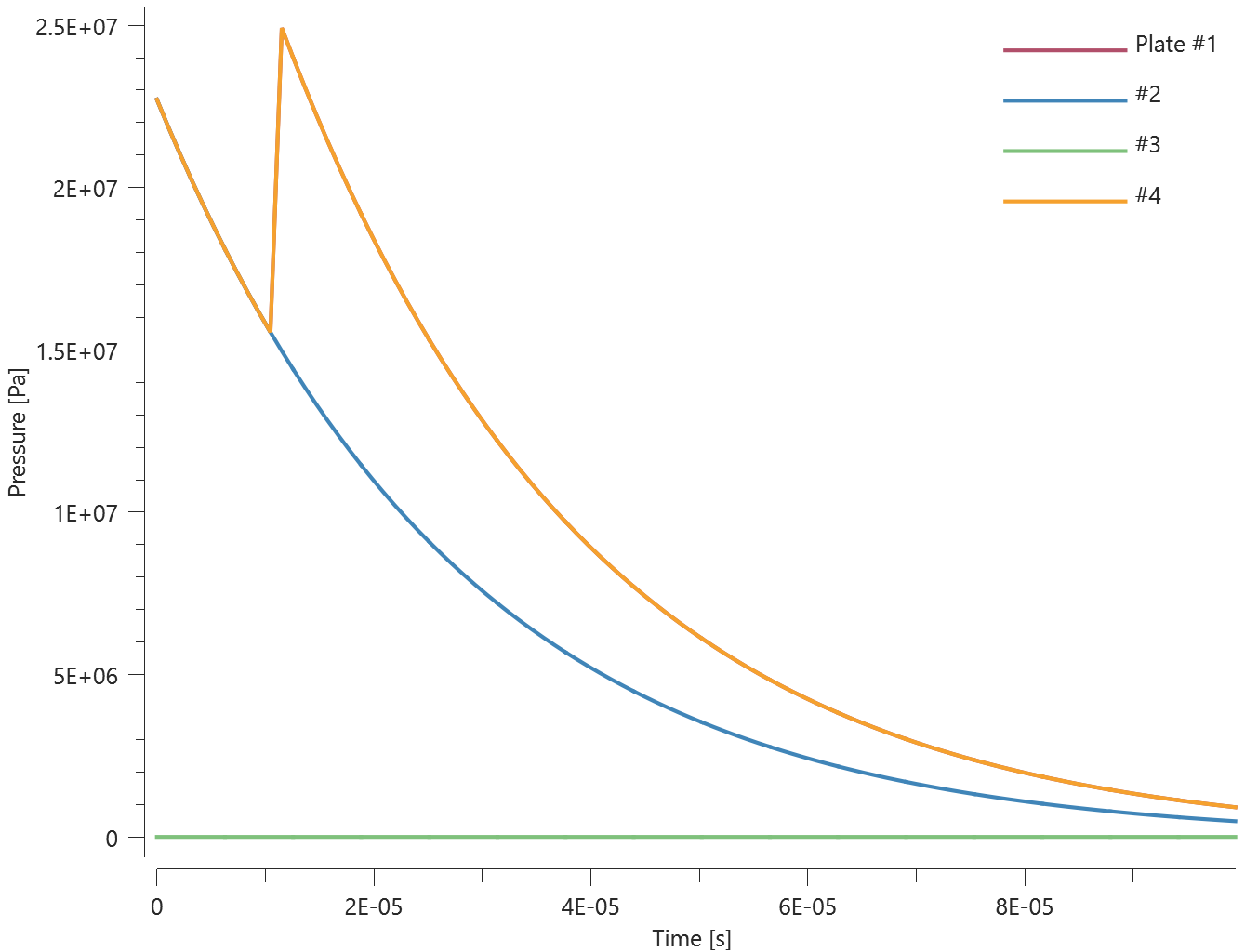
Tests
This benchmark is associated with 1 tests.
Reflective pressure
"Optional title"
coid
entype, enid, $mtnt$, $x_c$, $y_c$, $z_c$, tid, diffract
toff, ground, $t_{end}$
The model consists of a spherical charge and eight quadratic plates. The plates are distributed around the explosive charge with their normal directions coinciding with the direction of propagation of the blast wave. The distance between the plates and the explosive charge differs for each plate. An illustration of the test setup is presented in Figure 1.
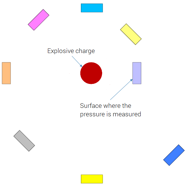
The peak reflective pressure at eight different scaled distances in the range of $0.5 - 10$ is compared to emperical data from M. Swisdak, Jr, (1994) [1]. The comparison is displayed in Figure 2 and 3.
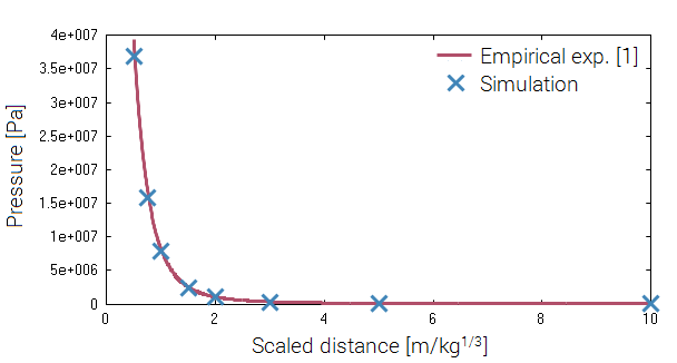
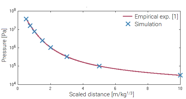
Reference
[1] - Swisdak M. (1994), Simplified Kingery Airblast Calculations, Naval Surface Warfare Center.
Tests
This benchmark is associated with 1 tests.
Underpressure
"Optional title"
coid
entype, enid, $mtnt$, $x_c$, $y_c$, $z_c$, tid, diffract
toff, ground, $t_{end}$
This model tests the *LOAD_AIR_BLAST command. One box (*COMPONENT_BOX) and one charge (*LOAD_AIR_BLAST) is positioned as displayed in Figure 1. Surface pressure is measured with a sensor positioned at the center of the surface that is facing the charge.
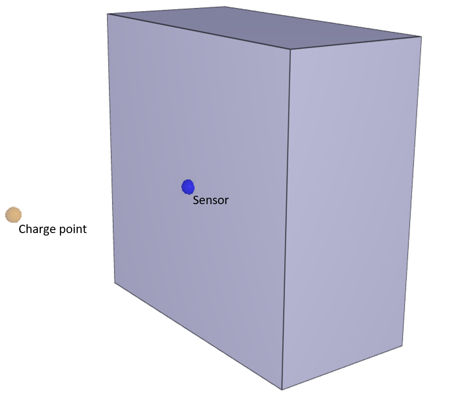
The test should result in a rapid increase in pressure followed by an exponential decay to the ambient pressure and a longer phase of negative pressure. See Figure 2.
Target:
-There should be an underpressure phase in the test i.e. p<0
Maximum, minimum and average value of pressure at the sensor is checked for version control.
Tests
This benchmark is associated with 1 tests.
*LOAD_CENTRIFUGAL
Centrifugal forces
"Optional title"
entype, enid, cid, csysid, $t_{beg}$, $t_{end}$
This tests the *LOAD_CENTRIFUGAL command. A centrifugal force is loaded to a rigid sphere with a radius of $r = 0.1 \ m$ and a density of $\rho= 1000 \ kg/m^3$. The force is applied in a local coordinate system.
Rigid body mass:
$$ m = \frac{\rho\cdot 4\pi r^3}{3} = 4.1888 \ kg $$
Vector from COG to spin axis:
$$ \tilde{r} = [0, 0, 2] $$
Spin vector:
$$ \tilde{\omega} = 10 \cdot [0.8, 0.5, 0.33166] $$
Resulting force:
$$ \tilde{F} = -m \times [\tilde{\omega} \times [\tilde{\omega} \times \tilde{r}]] = [-222.3, -138.9, 745.6] \ N $$
The resulting force values found in "rigid.out" and in "prescribed.out" is being checked for version control.
Tests
This benchmark is associated with 1 tests.
*LOAD_DAMPING
Different element polynomial order
"Optional title"
entype, enid, cid, $\mu$, $c_{dec}$, $sf$, gid
This model tests the *LOAD_DAMPING command. Damping is applied to linear, quadratic and cubic hex elements.
| Mass proportinal damping: | $F = -C \cdot m \cdot v$ |
| Damping coefficient: | $C = 2$ |
| Initial velocity $(x_{axis})$: | $1 \ m/s$ |
| Velocity at time $t$: | $v(t) = v_{0} \cdot exp(-C \cdot t)$ |
| At termination $(t=1)$: | $v(1) = v_{0} \cdot exp(-C) = 0.13534 \ m/s$ |
The velocity is tested against results in "rigid.out" and in "part.out".
Tests
This benchmark is associated with 1 tests.
Mass damping
"Optional title"
entype, enid, cid, $\mu$, $c_{dec}$, $sf$, gid
Tested parameters: entype, enid, cid, $sf$.
This model tests the mass damping parameters in the command *LOAD_DAMPING. The test consists of an elastic cantilever beam that is exposed to a static pressure load.
Mass damping is used to approach the static equilibrium. The load applied is a distrubuted load of $10 \ kPa$. See Figure 1.
The mass damping force $F_{i}$ acting on node $i$ is:
$$ F_{i} = \Bigg\{ \begin{array}{ll} \ \hspace{10pt} -C \cdot m_{i} \cdot v_{i} \hspace{10pt} : \hspace{10pt} When \ moving \ towards \ equilibrium\\ -sf \cdot C \cdot m_{i} \cdot v_{i} \hspace{10pt} : \hspace{10pt} When \ moving \ away \ from \ equilibrium\\ \end{array} $$
where $C$ is the damping coefficient defined with a CURVE or FUNCTION with ID cid, $m_{i}$ is the node mass, $v_{i}$ is the node velocity and $sf>1$ is a mass damping scale factor which is used for faster dynamic relaxation.
The scale factor is only activated when moving away from equilibrium which is automatically determined from the energy levels.
For comparison, to see the effect of mass damping, three equaivalent beams are tested for with different values for $C$ and $sf$. See Figure 2.
Sensors are placed at the center of the free ends of the beams to measure tip displacements.
The effect of the mass damping can be seen in Figure 3.
First, average, maximum and last values of tip displacements are checked for version control.
Tests
This benchmark is associated with 1 tests.
Viscous damping
"Optional title"
entype, enid, cid, $\mu$, $c_{dec}$, $sf$, gid
Tested parameters: entype, enid, $\mu$, $c_{dec}$.
The model tests the viscous damping parameters in the command *LOAD_DAMPING. The test consists of two tip loaded cantilever beams, one with applied viscous damping and one without. See Figure 1.
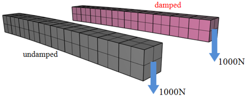
Two output sensors are placed at the center of the free ends of the beams to measure tip displacement. The effect of damping for the undamped compared to the damped beam can be seen in Figure 2.
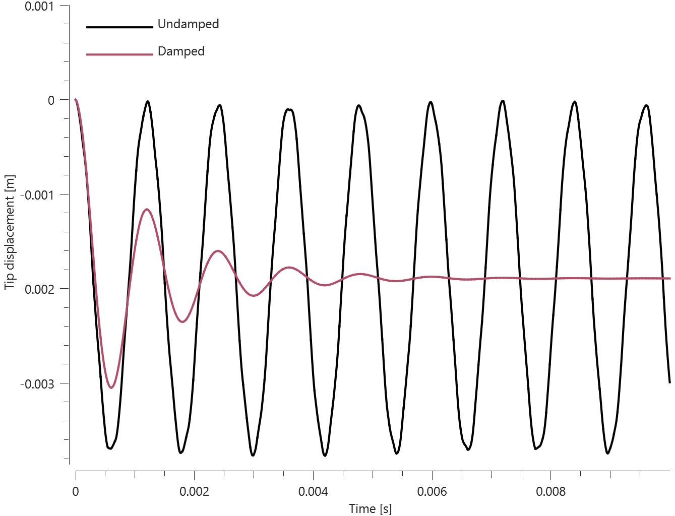
First, average and last values of tip displacements are checked for version control.
Tests
This benchmark is associated with 1 tests.
*LOAD_ELEMENT_SMOOTHING
Version control
"Optional title"
coid
entype, enid, $t_{dec}$
This tests the *LOAD_ELEMENT_SMOOTHING command.
A rubber block is impacted by a rigid pipe. Element smoothing is applied to suppress the development of high frequency noise on element level.
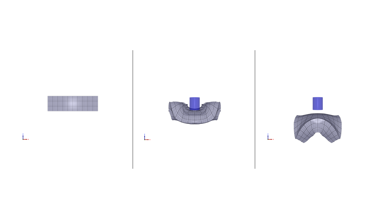
An output sensor is placed at the center of the block on the top. From the sensor the volumetric strain is measured, and values for maximuim and average volumetric strain is checked.
Tests
This benchmark is associated with 1 tests.
*LOAD_EM_CABLE
Curvature
"Optional title"
coid
pid$_{1}$, pid$_{2}$, fid$_{1}$, fid$_{2}$
This test the maximum curvature of a cable using *LOAD_EM_CABLE command.
A rigid circular pipe is created with a separate cable inside. Both the pipe and the cable is exposed to an electromagnetic force.
The curvature is defined as $1/R$, where $R$ is the radius of the curvature. Since the pipe is rigid the curvature can be calculated using its given radius. The caluculated value is then compared to the simulation. Setup of the test can be seen in Figure 1.
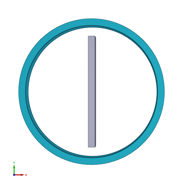
The maximum radius of the pipe is checked.
Tests
This benchmark is associated with 1 tests.
Electromagnetic force
"Optional title"
coid
pid$_{1}$, pid$_{2}$, fid$_{1}$, fid$_{2}$
This tests the *LOAD_EM_CABLE command.
Two long cables are created using *COMPONENT_BOX. The two cables are both given an current each, and an analytical result for the force per unit length is calculated. The analytical result is then compared to the force obtained from the simulation.
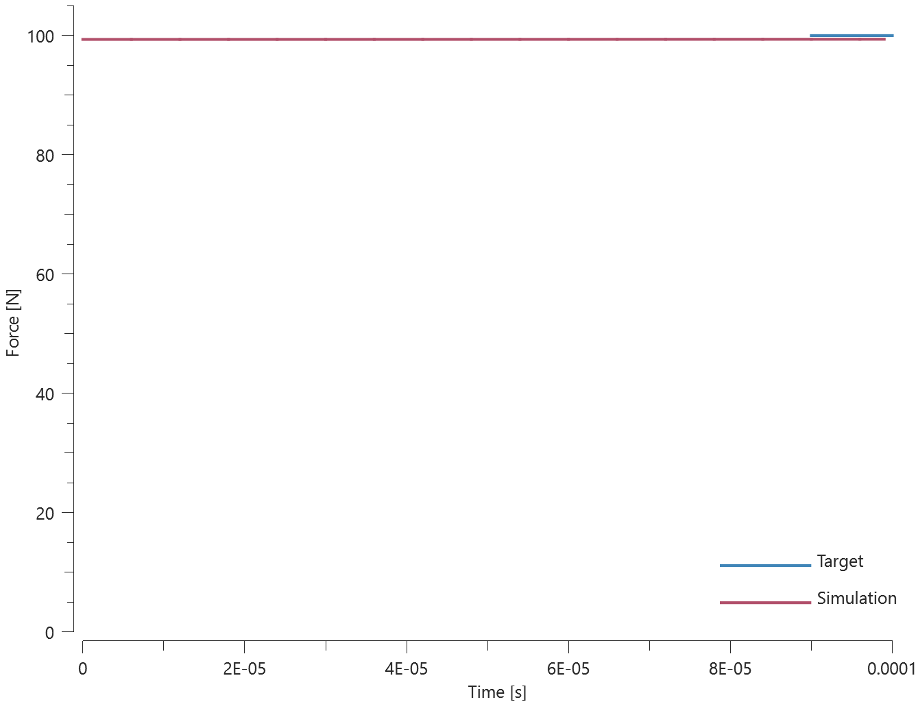
Maximum force in Y-direction is checked against the analytical result.
Tests
This benchmark is associated with 1 tests.
*LOAD_FORCE
Load on box
"Optional title"
coid
entype, enid, direc, cid, $sf$, csysid, $t_{beg}$, $t_{end}$
This tests the *LOAD_FORCE command. The subject is a rigid body with a mass of $1 \ kg$.
*GEOMETRY_SEED_COORDINATE is used to specify the loaded nodes. The force is applied in a local coordinate system, with a scale factor ($sf$), and with a birth and death time - both of which are within the time frame of the simulation.
A sine function gives the magnitude of the force:
$$ \lvert F\rvert = sf\cdot sin(\pi \cdot t)\hspace{40pt} t\in [0.1,0.2] $$
Which gives a total impulse of:
$$ \int\limits_{0.1}^{0.2} sf\cdot sin(\pi t) dt = 0.0045213 $$
The final velocity is:
$$ \tilde{v}_{end} = 0.0045213 \cdot [1,1,0]/\sqrt{2} = [0.00319, 0.00319, 0] $$
The velocity found in "rigid.out" and in "part.out" is being checked for version control.
Tests
This benchmark is associated with 1 tests.
*LOAD_FORCE_INTERACT
Magnetic field
"Optional title"
coid
entype${}_1$, enid${}_1$, entype${}_2$, enid${}_2$, fid, dtype, dynamic
Tested parameters: coid, entype${}_1$, enid${}_1$, entype${}_2$, enid${}_2$, fid.
This model tests the command *LOAD_FORCE_INTERACT.
A rectangular bar magnet that consists of a north and south pole is created with the command. It interacts with surrounding pieces of metals through its magnetic field which is constructed by applying a repelling force to the north pole and an attracting force to the south pole. See Figure 1.
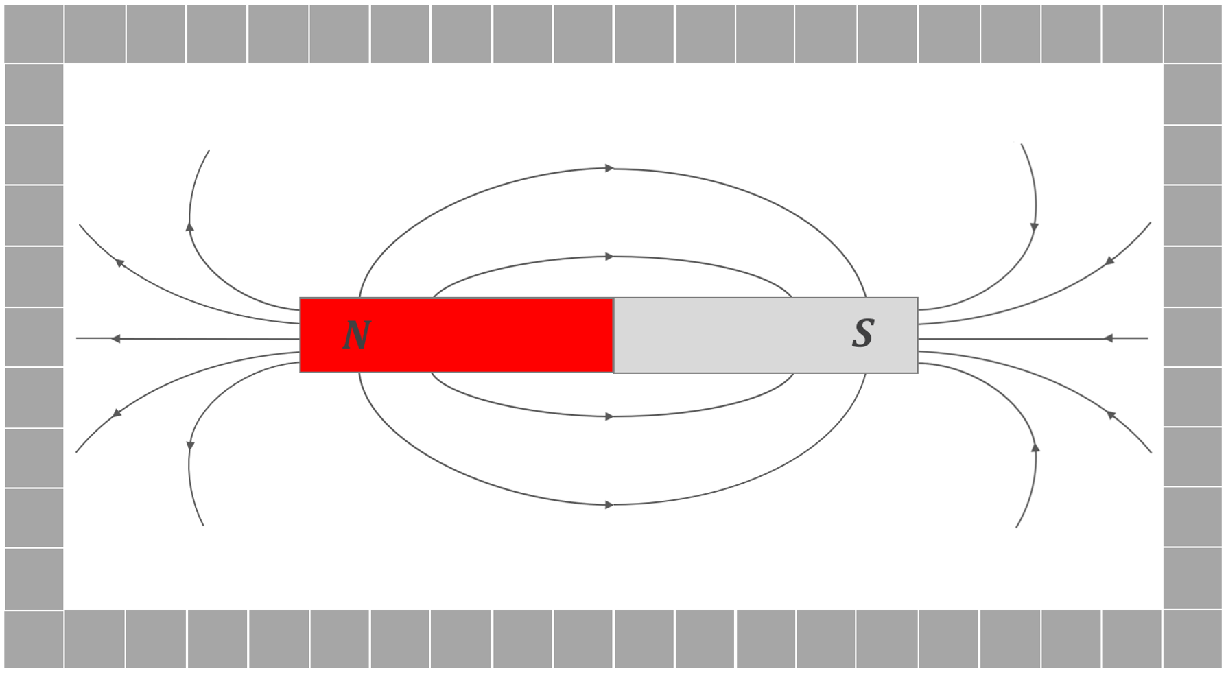
The force per unit body volume is defined by a FUNCTION with ID=fid. The relative location of the bodies defines the direction of the force. The magnitude of the force is allowed to depend on their relative distance (intrinsic variable dist).
$$ F = \frac{C}{dist^2} $$
Where the constant C can vary along the length of the magnet. Stronger at the ends and weaker closer to the center of the magnet. The accuracy can thus be increased by dividing the magnet into more elements which will distribute the force intensity further out to the ends.
The magnetic field from the test can be seen in Figure 2, where the path in X & Y-coordinates of the surrounding objects are plotted. The magnet is divided into 4 elements in total.
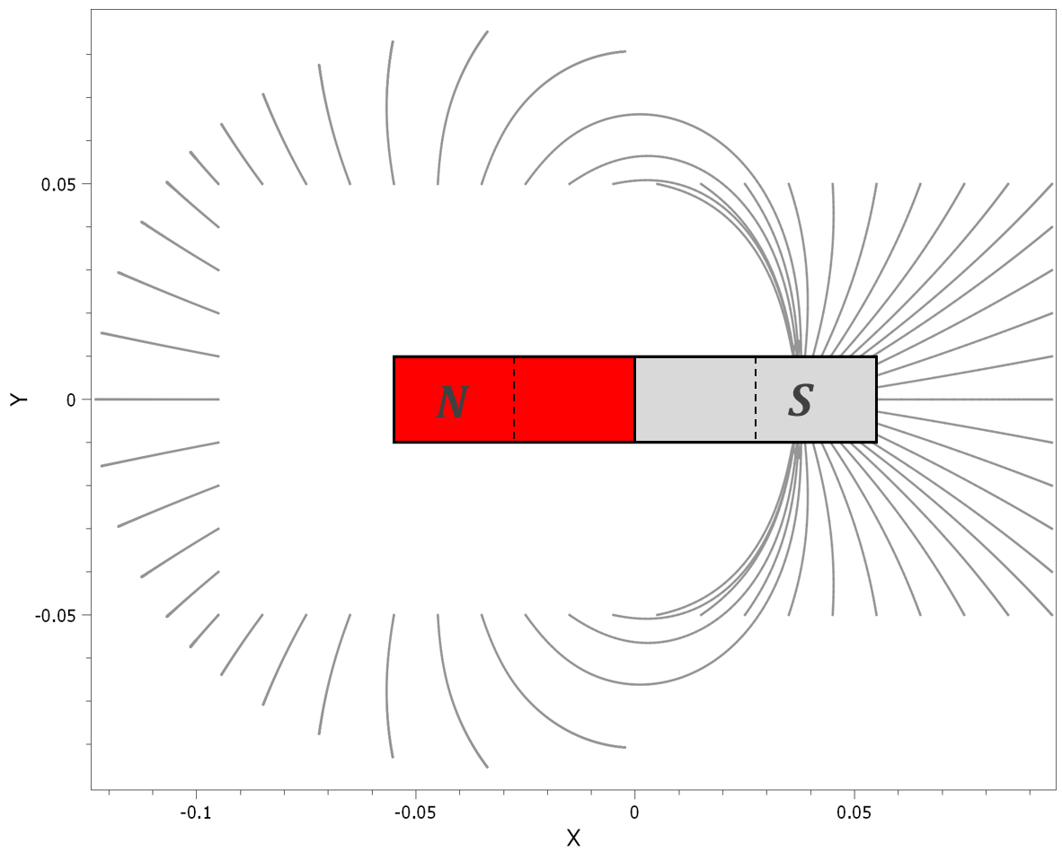
The result obtained from the simulation can be compared to a physical experiment where the magnetic field is revealed by iron filings on a paper. See Figure 3.
The last X & Y-coordinates of some selected cubes are checked for version control.
Reference
[1] - Newton Henry Black, Harvey N. Davis (1913) Practical Physics, The MacMillan Co., USA, p. 242, fig. 200
Tests
This benchmark is associated with 1 tests.
*LOAD_GRAVITY
Gravity test
"Optional title"
direc, cid, addmass, csysid, $sf$
This tests the *LOAD_GRAVITY command. All element types are tested in three simulations - one simulation for a gravity in each coordinate direction. The gravity constant is set to $10 \ m/s^{2}$, and the velocity at termination ($t=1$) should therefore be $10 \ m/s$.
The velocities are checked based on output in "rigid.out" and in "part.out".

Tests
This benchmark is associated with 3 tests.
Mass scaling (include and exclude added mass)
"Optional title"
direc, cid, addmass, csysid, $sf$
This model tests the option of including/excluding added mass due to mass scaling for the command *LOAD_GRAVITY. A cube of $1 \ kg$ is in contact with a rigid plate. Gravity in negative z-direction is acting on the model with a gravitational constant $g=10$. See Figure 1.
/mass_scaling_1.png)
Mass scaling is activated with maximum allowed mass scaling factor $ms_{max}=2$ in *TIME.
To control the added mass due to mass scaling from gravity loading, the parameter "addmass" is set to either 0 (include added mass) or to 1 (exclude added mass). The contact force between the cube and the plate should be:
Excluding added mass: $F = m \cdot a = 1 \cdot 10 = 10 \ N$
Including added mass: $F = m \cdot a = (m_{original} + m_{added}) \cdot a = 2 \cdot 10 = 20 \ N$
Contact force is checked for version control.
Tests
This benchmark is associated with 2 tests.
*LOAD_PRESSURE
Load in part geometry
"Optional title"
coid
entype, enid, cid, $sf$, $t_{beg}$, $t_{end}$, csysid, gid${}_{SPH}$
This tests the *LOAD_PRESSURE command. A shell structure modeled by one layer of cubic hexahedral elements is loaded by a triangular pressure time curve. To load only a part of the structure, a patch of shell elements with a defined thickness is created. The patch is positioned so that its thickness covers a part of the structures surface. The command *GEOMETRY_PART is then used to define a geometry equivalent to the patch and this geometry is loaded by *LOAD_PRESSURE. A figure of a simplified case of this test is presented in Figure 1.
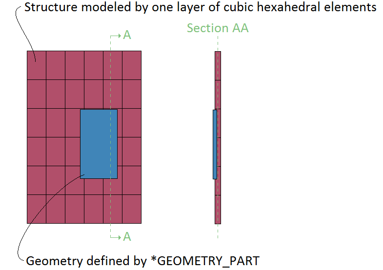
The pressure functionality applies to complete element surfaces and surfaces are included in the defined geometry provided that the element surface centroid is within the geometry. This holds regardless of the polynomial order used in the elements. It is therefore important to pay attention to how the geometry covers the mesh-grid. As for the case illustrated in Figure 1, the pressure will operate as illustrated in Figure 2.
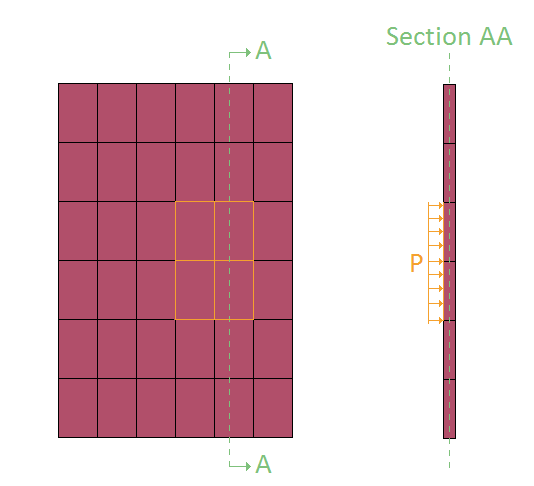
The following conditions were used:
| End time of simulation: | $t_{end} =0.01 \ s$ |
| Max pressure, at $t_{end}/2$: | $p_{max} = 4 \ MPa$ |
| Area of shell in yz-plane: | $A_{patch} = 3.603 m \cdot 3.023 m = 10.89 \ m^{2}$ |
| Target momentum transfer in x-direction: | $= A_{patch} \cdot \dfrac{p_{max}\cdot t_{end}}{2}= 2.18e^{5} \ Ns$ |
The momentum is output to "part.out", which is checked for version control.
Tests
This benchmark is associated with 1 tests.
Load on rigid body
"Optional title"
coid
entype, enid, cid, $sf$, $t_{beg}$, $t_{end}$, csysid, gid${}_{SPH}$
This tests the *LOAD_PRESSURE command. The pressure is applied to rigid elements of all element types. The command is used with a scale factor and a birth- and death time. For version control, final velocities are checked.
| Parts thickness (y-direction): | $d = 0.1 \ m$ |
| Material density: | $\rho = 1000 \ kg/m^{3}$ |
| Area density: | $\rho_{A} = d\cdot \rho = 100 \ kg/m^{2}$ |
| Pressure level: | $p = sf\cdot 1 Pa = 7 \ Pa$ |
| Pressure active at: | $t \in [0.1,0.2]$ |
| Impulse per unit area: | $I = p\cdot (t_1 - t_0) = 0.7 \ Ns/m^{2}$ |
| Resulting velocity in y-direction: | $v_y = I\rho_A = 0.007 \ m/s$ |
The velocities are checked against output found in "part.out" and in "rigid.out".

Tests
This benchmark is associated with 1 tests.
Load on surface
"Optional title"
coid
entype, enid, cid, $sf$, $t_{beg}$, $t_{end}$, csysid, gid${}_{SPH}$
This model tests the *LOAD_PRESSURE command. A shell is loaded by a triangular pressure time curve. To load the entire shell, the *GEOMETRY_SEED_COORDINATE feature is applied to a coordinate on the shell surface. The total momentum transfer in X- and Y-direction (targets in Equations below) is checked for version control.
$$ A_x \cdot \dfrac{p_{max}\cdot t_{end}}{2}= 3.86 \ Ns $$
$$ A_y \cdot \dfrac{p_{max}\cdot t_{end}}{2}= 5.04 \ Ns $$
The max pressure is checked as well, and should occur half way through the simulation. The set-up parameters used are listed below.
| End time of simulation: | $t_{end} =0.01 \ s$ |
| Max pressure, at $t_{end}/2$: | $p_{max} = 4 \ MPa$ |
| Area of shell in yz-plane: | $A_x = 185.15 \ m^{2}$ |
| Area of shell in xz-plane: | $A_y = 25.19 \ m^{2}$ |
The momentums are output to "part.out" and max pressure to "sensor.out", all of which are checked for version control.
Tests
This benchmark is associated with 1 tests.
*LOAD_SHEAR
All element types
"Optional title"
entype, enid, cid${}_\tau$, cid${}_{vx}$, cid${}_{vy}$, cid${}_{vz}$, $t_{beg}$, $t_{end}$
This tests the *LOAD_SHEAR command. A shear load is applied to act in positive X-direction on all element types. The load is applied to faces with normals in positive and negative Y-direction.
| Parts thickness (y-direction): | $d = 0.1 \ m$ |
| Material density: | $\rho = 100 \ kg/m^{3}$ |
| Area density: | $\rho_{A} = d\cdot \rho = 10 \ kg/m^{2}$ |
| Initial relative velocity: | $v_{0} = 3 m/s \ $ |
| Shear traction (x-direction): | $t_{x} = C\cdot v_{tang} $ |
| Shear active at: | $\in [0.1,0.2]$ |
| Acceleration in x-direction:: | $a_{x} = -\frac{d}{dt}(v_{tang}) = 2\frac{t_x}{\rho_A} = 2C\cdot \frac{v_{tang}}{\rho_A} = 0.4v_{tang}$ |
Solving the differential equation gives the final velocity in X-direction:
$$ v_x = v_0(1 - \exp\dfrac{-2C(t_1-t_0)}{\rho_A}) = {3(1 - \exp(-0.04))} = 0.11763 \ m/s $$
The velocities are checked against data found in "part.out" and in "rigid.out".
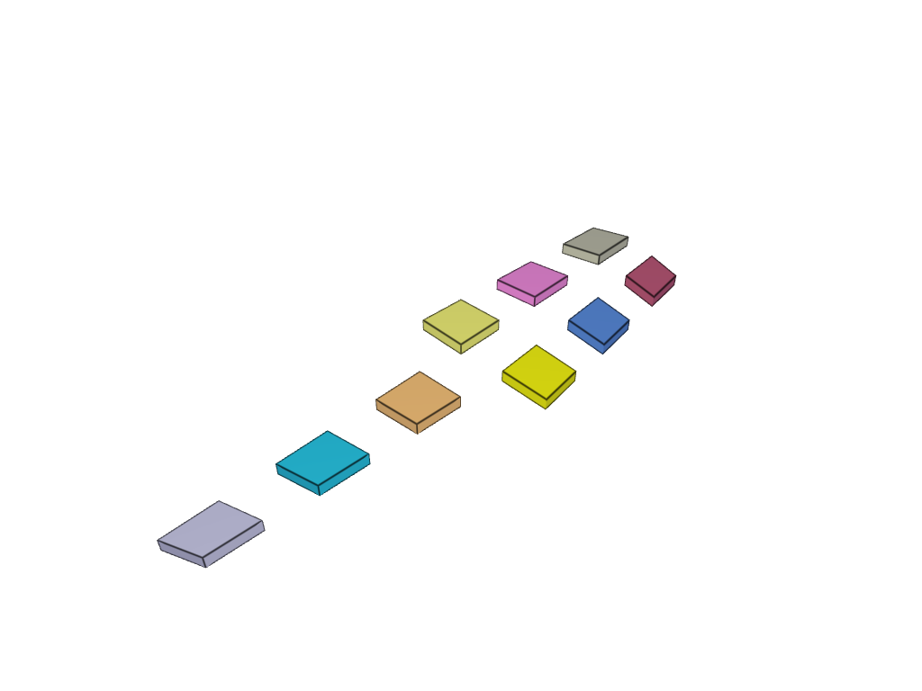
Tests
This benchmark is associated with 1 tests.
*LOAD_THERMAL_BODY
All element types
"Optional title"
coid, entype, enid, cid${}_1$, $sf$, $t_{beg}$, $t_{end}$, cid${}_2$
This tests the *LOAD_THERMAL_BODY command. A thermal load is applied to 9 bodies: all element types are tested.
| Thermal body load: | $Q = sf\cdot Q_0 = 2000 \ W$ |
| Heat capacity: | $C_p = 100 \ J/K$ |
| Density: | $\rho = 1 \ kg/m^{3}$ |
| Deposited heat: | $W = Q(t_1-t_0) = 200 \ J/m^{3}$ |
| Temperature increase: | $dT = W/(\rho\cdot C_p) = 200/100 = 2 \ K $ |
The final temperature for all elements is checked for version control.

Tests
This benchmark is associated with 1 tests.
*LOAD_THERMAL_RADIATION
Cooling plate
"Optional title"
coid
entype, enid, $T_{amb}$, $d_{max}$, $\Delta t_{update}$
Tested parameters: coid, entype, enid, $T_{amb}$.
The thermal radiation properties in *LOAD_THERMAL_RADIATION is verified in this test.
A quadratic plate with side length $200 \ mm$ and thickness $20 \ mm$ is given an initial temperature of $1273.15 \ K$ $(1000°C)$. The ambient temperature surrounding the hot plate is $273.15 \ K$ $(0°C)$. For $100$ seconds the plate is cooling off in the surrounding temperature.
The test setup is displayed in Figure 1.
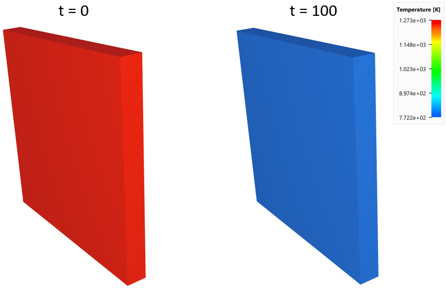
To simplify the test, the heat conductivity is set to a high value, for a homogeneous temperature response throughout the plate. Thermal emissivity is set to $1$ and the heat capacity $400 \ J/K$. The density of the material is $3000 \ kg/m^3$.
Temperature vs. time and thermal energy vs. time from the simulation is presented in Figure 2 and 3 together with target curves from a verification script.
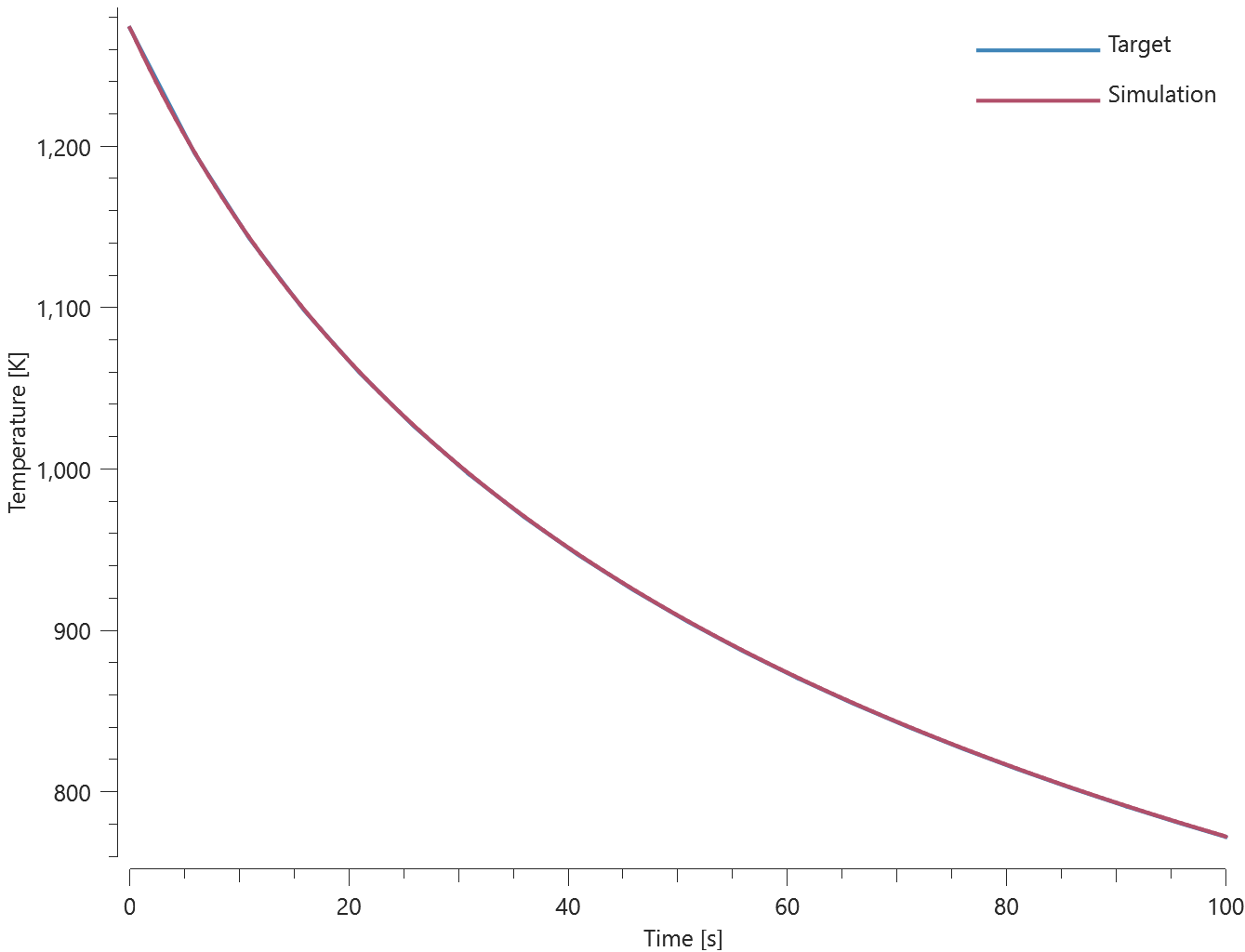
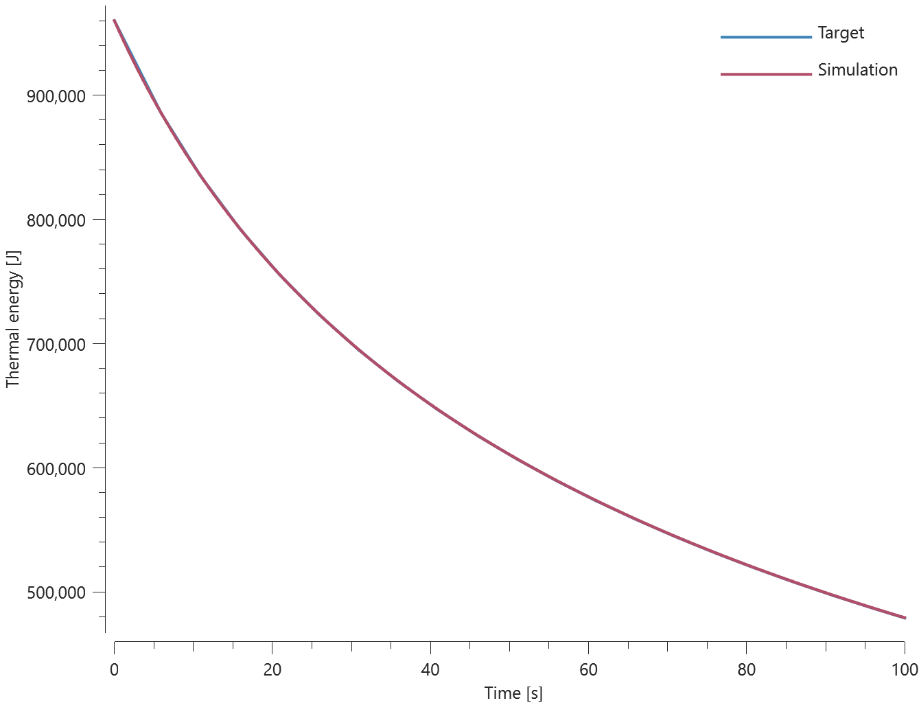
First, average and last values for temperature and thermal energy is checked for version control.
Tests
This benchmark is associated with 1 tests.
Interaction test
"Optional title"
coid
entype, enid, $T_{amb}$, $d_{max}$, $\Delta t_{update}$
Tested parameters: coid, entype, enid, $T_{amb}$.
This model tests the thermal radiation and interaction between a hot and a cold plate with the command *LOAD_THERMAL_RADIATION.
The test consists of two quadratic plates with side length $200 \ mm$ and thickness $20 \ mm$. The hot plate is given an initial temperature of $1273.15 \ K$ $(1000°C)$ and the cold plate $273.15 \ K$ $(0°C)$. The ambient temperature in the surrounding is $273.15 \ K$ $(0°C)$.
Simulation time is set to $100$ seconds and at the beginning the plates are at a distance of $20 \ mm$, perpendicular from one another. For the duration the plates are moving away from one another at a constant velocity of $2 \ mm/s$. The emissivity of the cold plate is low and a significant amount of energy is reflected back to the hot plate.
The test setup is displayed in Figure 1.
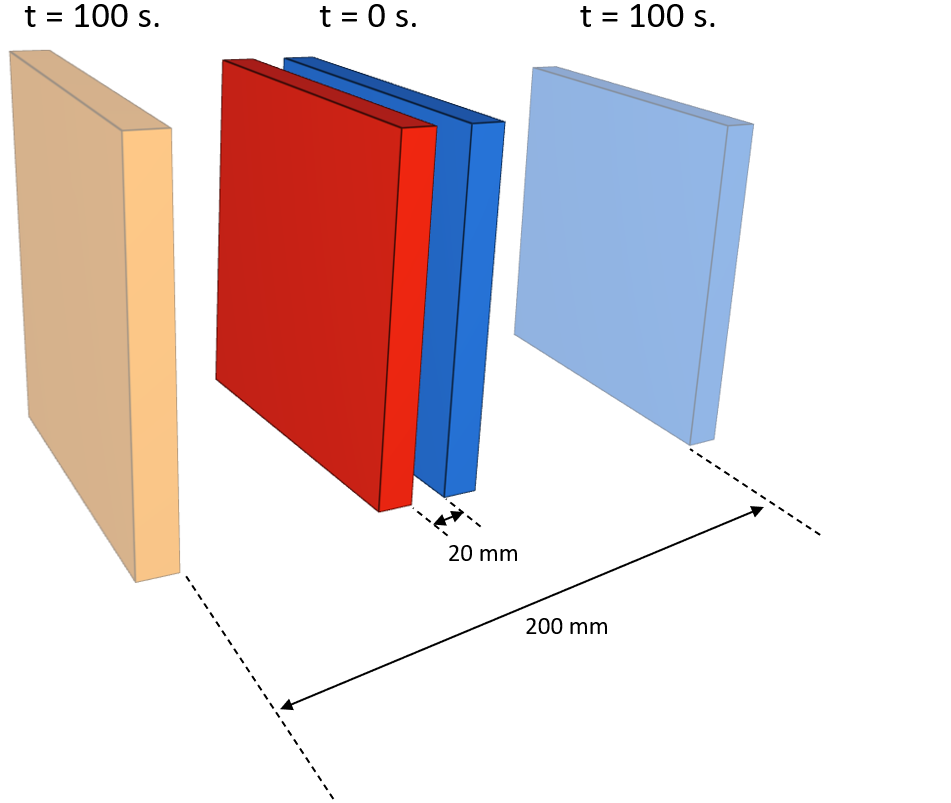
To simplify the test, the heat conductivity is set to a high value, for a homogeneous temperature response throughout the plate.
Thermal emissivity, $\epsilon$, is set to $1$ for the hot plate and $0.1$ for the cold plate.
Heat capacity is set to $400 \ J/K$.
Density of the material is $3000 \ kg/m^3$.
Temperature vs. time and thermal energy vs. time for the hot plate is presented in Figure 2 and 3 together with target curves from a verification script.
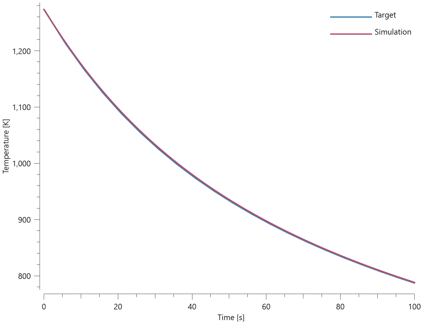
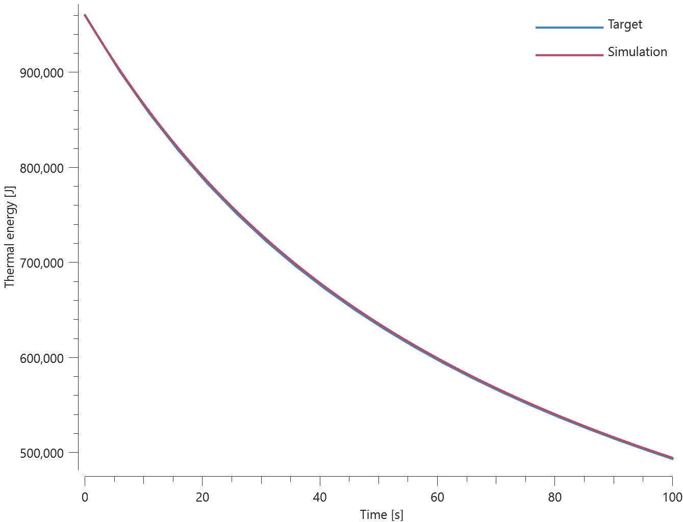
First, average and last values for temperature and thermal energy is checked for version control.
Tests
This benchmark is associated with 1 tests.
Temperature dependent specific heat capacity
"Optional title"
coid
entype, enid, $T_{amb}$, $d_{max}$, $\Delta t_{update}$
This test verifies that a temperature dependent specific heat capacity (specified in *PROP_THERMAL) can be used with *LOAD_THERMAL_RADIATION.
A linear element with an initial temperature of $1000 \ K$ and a temperature dependent specific heat capacity is defined. A high thermal conductivity is specified, meaning that the spatial variation in element temperature is negligable. The ambient temperature is set to $293 \ K$. Element temperature vs. time from the simulation is presented in Figure 1 together with target curves from a verification script.
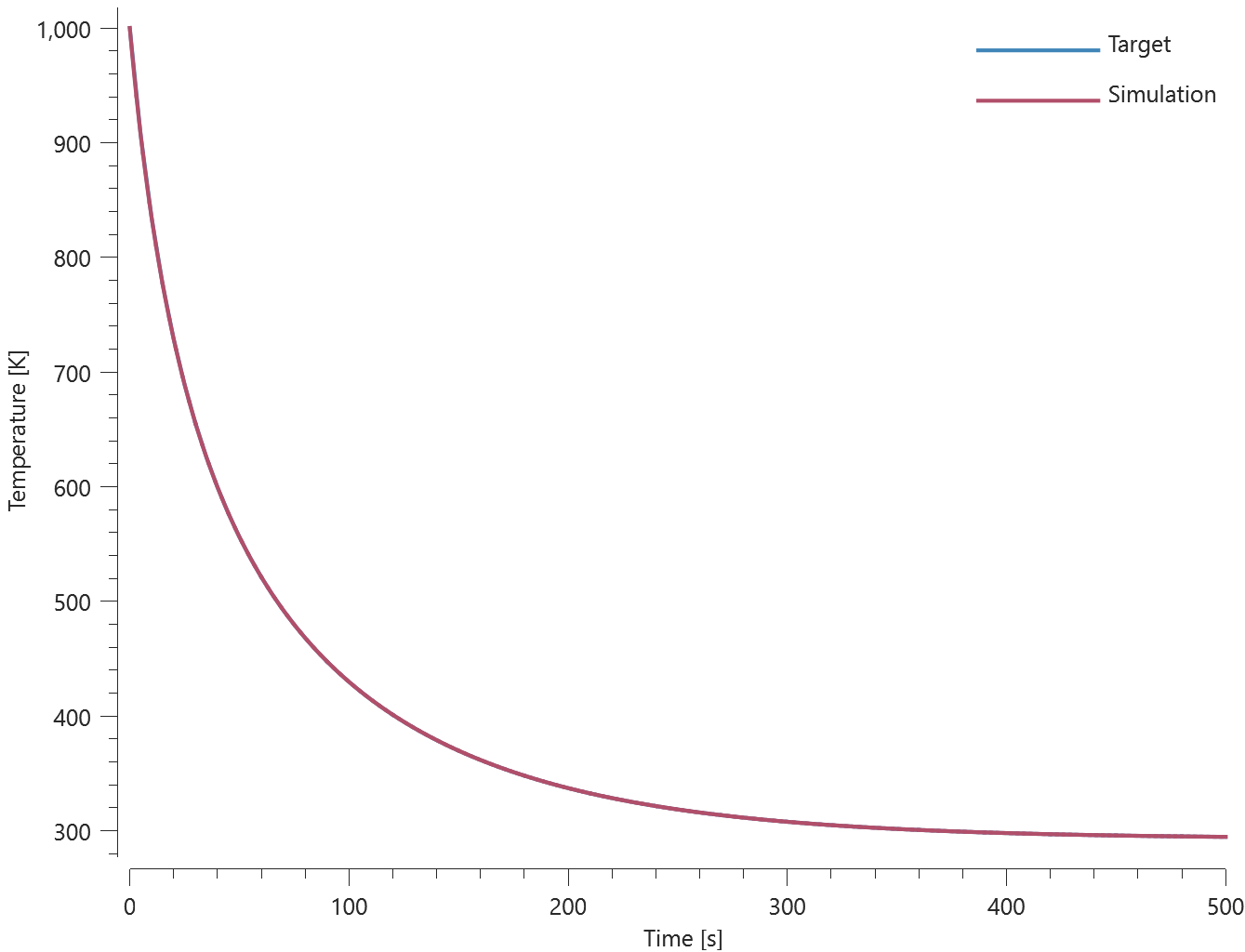
Initial, final and average temperature is checked.
Tests
This benchmark is associated with 1 tests.
*LOAD_THERMAL_SURFACE
All element types
"Optional title"
coid, entype, enid, cid, $sf$, $t_{beg}$, $t_{end}$
This tests the *LOAD_THERMAL_SURFACE command. A thermal load is applied to 9 surfaces: all element types are tested. The thermal surface load is applied to faces with normals in positive Y-direction. Heat conduction will eventually distribute the temperature evenly to all elements.
| Thermal surface load: | $Q = sf\cdot Q_0 = 2000 \ W/m^{2}$ |
| Heat capacity: | $C_p = 100 \ J/K$ |
| Heat conductivity: | $k = 1 \ W/mK$ |
| Density: | $\rho = 1 \ kg/m^{3}$ |
| Material thickness: | $t = 0.1 \ m$ |
| Area density: | $\rho_A = \rho \cdot t = 0.1 \ kg/m^2$ |
| Deposited heat per unit area: | $W = Q(t_1-t_0) = 200 \ J/m^2$ |
| Temperature increase: | $dT = W/(\rho_A\cdot C_p) = 200/10 = 20 \ K$ |
The final temperature is checked for version control.

Tests
This benchmark is associated with 1 tests.
*LOAD_UNDEX
Geers Hunter
"Optional title"
coid
entype, enid, $x_c$, $y_c$, $z_c$, gdir, $d$
$m_{HE}$, $\rho_{HE}$, $p_c$, $v_c$, $A$, $B$, $\gamma$, $K_c$
$C_d$, $E_d$, $\dot{u}_0$
The command *LOAD_UNDEX is mainly based on equations presented in T. L. Geers & K. S. Hunter (2002) [1].
Underwater explosions are modeled in two phases: a shock-wave phase and an oscillation phase. The shock-wave phase is significantly shorter in time compared to the oscillation phase. Initial conditions for the oscillation phase are set based on the conditions at the end of the shock-wave phase.
An octave script is created to verify the command *LOAD_UNDEX. This script is created based solely on the referenced article and verified by re-creating some relevant figures from the article.
Pressure vs time (non-dimensionalized) from the similitude relation is presented in Figure 1.
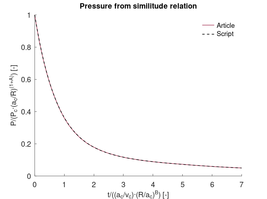
Initial conditions for the oscillation phase are to be selected at a time when the pressure is reduced to 5-10% of its peak value, i.e., time between 3 – 7 in Figure 1. Bubble radius vs. time (non-dimensionlized) for this time interval is presented in Figure 2. Bubble radius and its first and second time derivative are used as initial conditions in the oscillation phase.
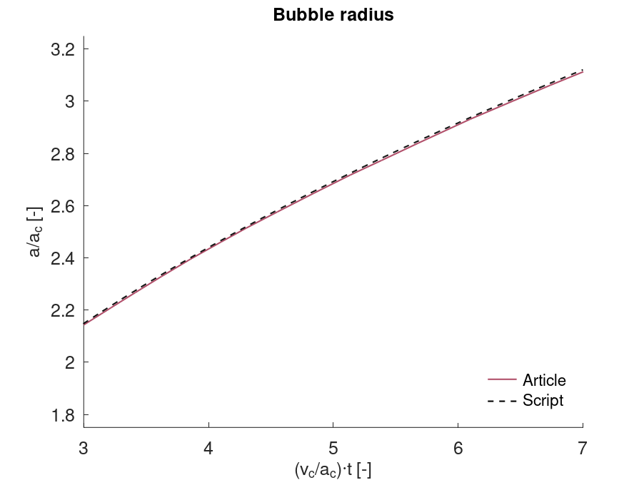
Bubble radius vs. time from the oscillation phase is presented in Figure 3 Initial conditions were selected at a non-dimensionalized time of 7 for this case.
The script is then used to verify the command *LOAD_UNDEX. The configuration is a $300 \ g$ charge detonated at a depth of $100 \ m$.
Bubble radius vs time is presented in Figure 4. Gas pressure in the bubble vs. time is presented in Figure 5 and Figure 6. Incident pressure $10 \ m$ from the center of the charge vs time is presented in Figure 7 and Figure 8. The Incident pressure is calculated based on the hyperacoustic case (eq. 4 in ref.) during the shock-wave phase, and the acoustic case during the oscillation phase (eq. 3 in ref.).
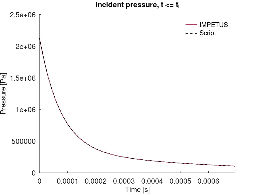
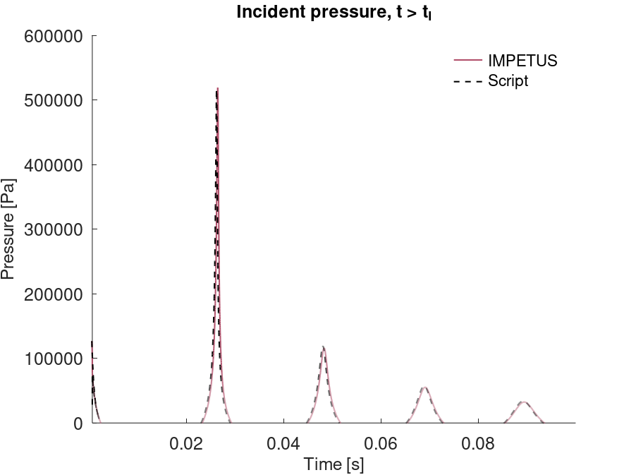
Reference
[1] T. L. Geers & K. S. Hunter, An integrated wave-effects model for an underwater explosion bubble, Journal of the Acoustical Society of America 111, 2002.
Tests
This benchmark is associated with 1 tests.
*MAP
Pressure loaded panel
"Optional title"
coid, $n_1$, $n_2$, $n_3$
$x_1$, ..., $x_8$
.
$x_M$, ..., $x_N$
This model tests the *MAP command.
A plate with side length $1 \ m$ and thickness $3 \ mm$ is subjected to load pressures of $1 \ MPa$. To apply the load pressure at wanted locations on the plate, the command *MAP is used.
The test is displayed in Figure 1.
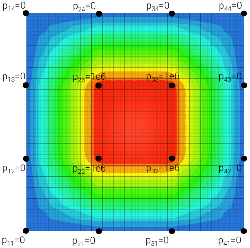
Two sensors are created to measure the applied pressure with targets:
- Sensor at $p_{11}$. Applied pressure should be $0 \ MPa$
- Sensor at center of plate. Applied pressure should be $1 \ MPa$
Tests
This benchmark is associated with 1 tests.
*MAT_BERGSTROM_BOYCE
Network A
"Optional title"
mid, $\rho$, $K$
$\mu$, $\lambda_L$, $a_0$, $a_1$, $\eta_\mathrm{max}$, $\dot{\gamma}_0$, $\xi$, $B$
$\sigma_0$, $Q$, $C$, $m$, $c_{dec}$, $\beta$, $W_c$, $\lambda_f$
$b_0$, $b_1$, $b_2$, $\mu_B$, erode
Network A in *MAT_BERGSTROM_BOYCE is verified in this test.
Tested parameters: $K$, $\mu$, $\lambda_L$, $a_0$, $a_1$ and $\eta_\mathrm{max}$.
A CHEX element is stretched in the X-direction while fixed in the Y- and Z-direction. Stress in the X-, Y- and Z-direction vs. volumetric strain from the element are presented in Figure 1 together with target curves obtained from a verification script.
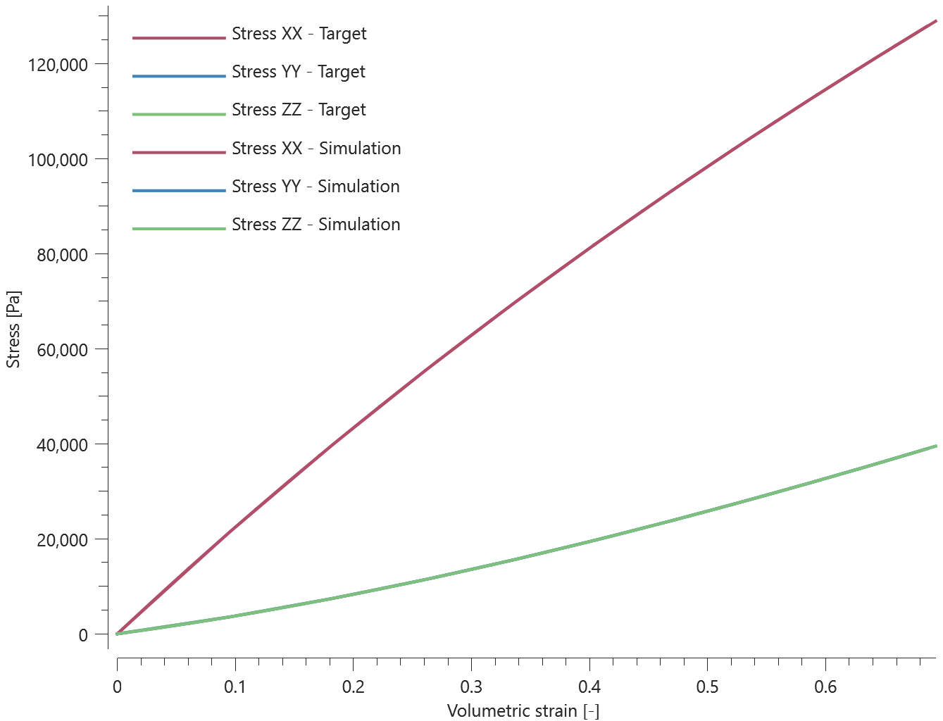
Maximum and average volumetric strain and stress in the X-, Y- and Z-direction are checked. The maximum Mullins/network damage is also checked.
Tests
This benchmark is associated with 1 tests.
Network A and B (alternative 2)
"Optional title"
mid, $\rho$, $K$
$\mu$, $\lambda_L$, $a_0$, $a_1$, $\eta_\mathrm{max}$, $\dot{\gamma}_0$, $\xi$, $B$
$\sigma_0$, $Q$, $C$, $m$, $c_{dec}$, $\beta$, $W_c$, $\lambda_f$
$b_0$, $b_1$, $b_2$, $\mu_B$, erode
Network A and Network B (alternative 2) in *MAT_BERGSTROM_BOYCE is verified in this test.
Tested parameters: $K$, $\mu$, $\lambda_L$, $a_0$, $a_1$, $\eta_\mathrm{max}$, $\dot{\gamma}_0$, $\xi$, $b_0$, $b_1$ and $b_2$.
A CHEX element is stretched in the X-direction while fixed in the Y- and Z-direction. Effective stress vs. volumetric strain in the element is presented in Figure 1 together with a target curve from a verification script.
/mat_bergstrom_boyce_network_A_and_B_alternative_2.png)
Maximum and average volumetric strain and effective stress are checked.
Tests
This benchmark is associated with 1 tests.
*MAT_CABLE
Failure model
"Optional title"
mid, $\rho$, $E$, $\nu$
$E_{t1}$, $E_{t2}$, $E_{tm}$, $\varepsilon_{tf}$, $\sigma_{ty}$
The material model *MAT_CABLE is verified in this test.
Tested parameters: $E$, $\nu$, $E_{t1}$, $E_{t2}$, $E_{tm}$, $\varepsilon_{tf}$, $\sigma_{ty}$.
In this test, two equivalent pipes on either side of the global X-axis are merged at their duplicated nodes creating a "cable". The cable is given a constant prescribed velocity at both ends generating tensile stresses. It is assigned the material model *MAT_CABLE and tensile fiber yield stress is set to $300 \ MPa$. A sensor is created in the middle of the cable.
The test setup is displayed in Figure 1.
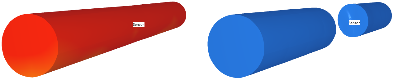
Targets:
- Maximum effective stress at sensor should be $300 \ MPa$
- Damage at sensor at $t_{end}$ should be $1$
Tests
This benchmark is associated with 1 tests.
Fiber stiffness
"Optional title"
mid, $\rho$, $E$, $\nu$
$E_{t1}$, $E_{t2}$, $E_{tm}$, $\varepsilon_{tf}$, $\sigma_{ty}$
The elastic parameters in *MAT_CABLE are verified in this test.
Tested parameters: $E$, $\nu$ and $E_f$.
Two CHEX elements are used in this test. One of the elements is loaded in tension and the other in compression. The elements are deformed in the X-direction while fixed in the Y- and Z-direction. The element in tension exhibits a higher stiffness due to the additional fiber stiffness term.
Stress in the X-, Y- and Z-direction vs. time from the elements are presented in Figure 1 and Figure 2 together with target curves from a verification script.
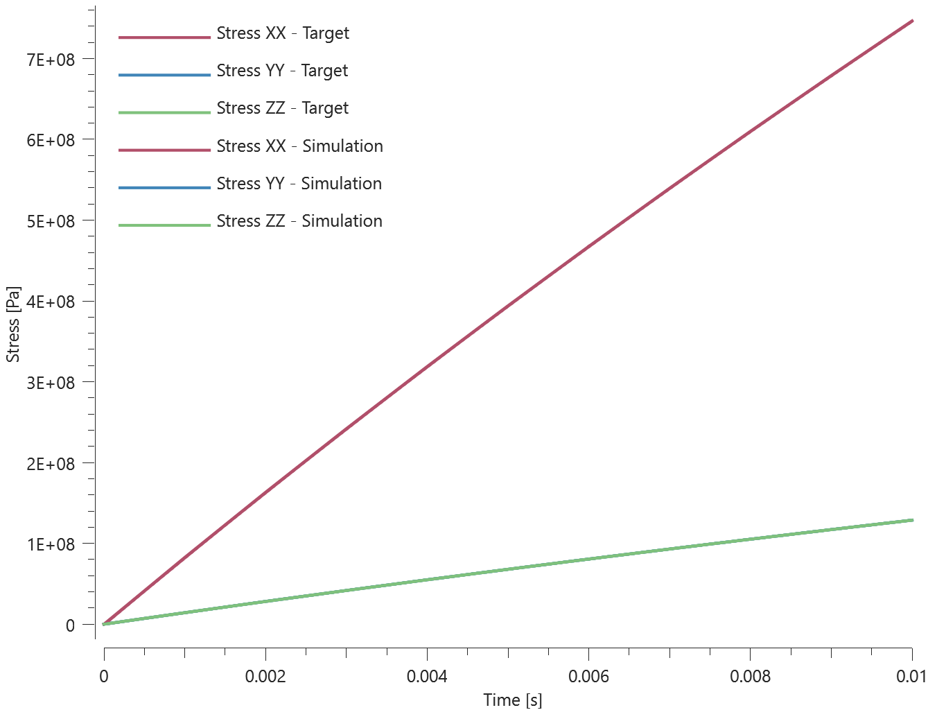
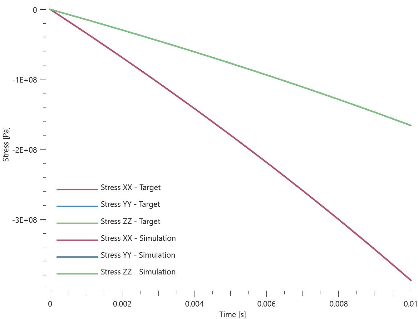
Maximum, minimum and average stress in X-, Y- and Z-direction are checked in the elements.
Tests
This benchmark is associated with 1 tests.
*MAT_CERAMIC
Crushing damage
"Optional title"
mid, $\rho$, $G$
$A_0$, $B_0$, $A_f$, $B_f$, $\varepsilon_f$, $\sigma_s$, $t_s$, $\alpha_s$
$K_1$, $K_2$, $K_3$, $\beta$, $K_c$, $\sigma_0^{max}$, $\sigma_f^{max}$
Crushing damage in *MAT_CERAMIC is verified in this test.
Tested parameter: $\varepsilon_f$.
A CHEX element is loaded in uniaxial compression. Crushing damage developes gradually based on the plastic strain:
$$ D_c = min\left(1.0, \frac{\varepsilon_{dev}^p}{\varepsilon_f}\right) $$
Crushing damage vs. effective plastic strain from the element is presented in Figure 1 together with a target curve from a verification script.
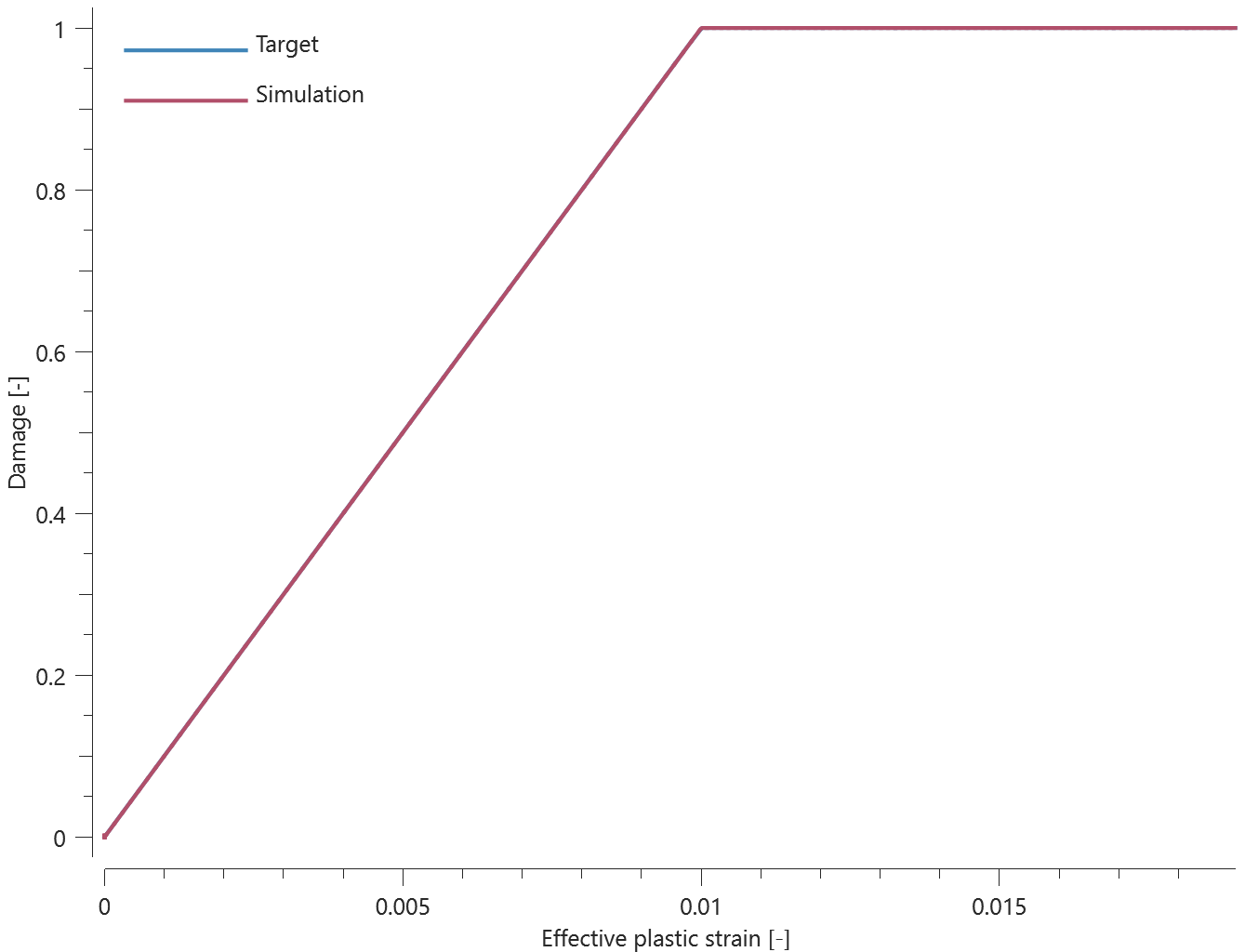
Maximimum and average damage and effective plastic strain are checked.
Tests
This benchmark is associated with 1 tests.
Direction of plastic flow
"Optional title"
mid, $\rho$, $G$
$A_0$, $B_0$, $A_f$, $B_f$, $\varepsilon_f$, $\sigma_s$, $t_s$, $\alpha_s$
$K_1$, $K_2$, $K_3$, $\beta$, $K_c$, $\sigma_0^{max}$, $\sigma_f^{max}$
The direction of plastic flow in *MAT_CERAMIC is verified in this test.
Tested parameter: $\beta$.
Two CHEX elements are compressed in the X-direction while fixed in the Y- and Z-direction. Parameter $\beta$ is set to $0$ in one of the elements and to $1$ in the other. The yield surface and failure surface coincides which means that the shear strength is not reduced with failure. Poisson's ratio is set to $0.0$ and the bulk modulus is defined as linear.
Yield strength, $\sigma_{y0}$:
$$ \sigma_{y0} = A_0 + B_0 \left(\frac{\sigma_{y0}}{3}\right) \implies \sigma_{y0}\left(1-\frac{B_0}{3}\right) = A_0 \implies \sigma_{y0} = \frac{A_0}{1-\frac{B_0}{3}} $$
Pressure at yield, $P_0$:
$$ P_0 = \frac{\sigma_{y0}}{3} $$
Volumetric strain at yield, $\varepsilon_{v0}$:
$$ \varepsilon_{v0} = -\frac{P_0}{K_1} $$
Volumetric strain at termination, $\varepsilon_{v}$:
$$ \varepsilon_{v} = log\left(1 + \frac{L-L_0}{L_0}\right) $$
where $L$ is the length at termination and $L_0$ the initial length.
Pressures at termination:
$$ P^{\beta = 0} = -K \varepsilon_{v} = -\frac{2}{3} G \varepsilon_{v} $$
$$ P^{\beta = 1} = P_0 - G \cdot (\varepsilon_{v} - \varepsilon_{v0}) $$
Effective stresses at termination:
$$ \sigma_{eff}^{\beta = 0} = A_0 + P^{\beta = 0} $$
$$ \sigma_{eff}^{\beta = 1} = A_0 + P^{\beta = 1} $$
Pressure vs. volumetric strain and effective stress vs. volumetric strain from both elements are presented in Figure 1 and 2 together with target curves based on the calculations above.
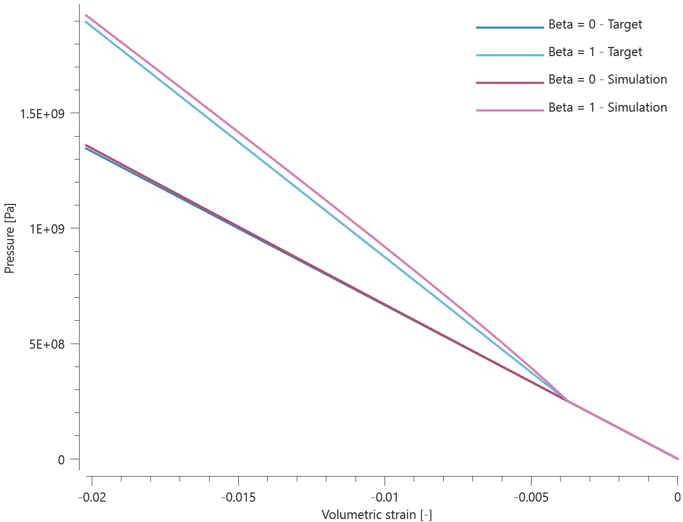
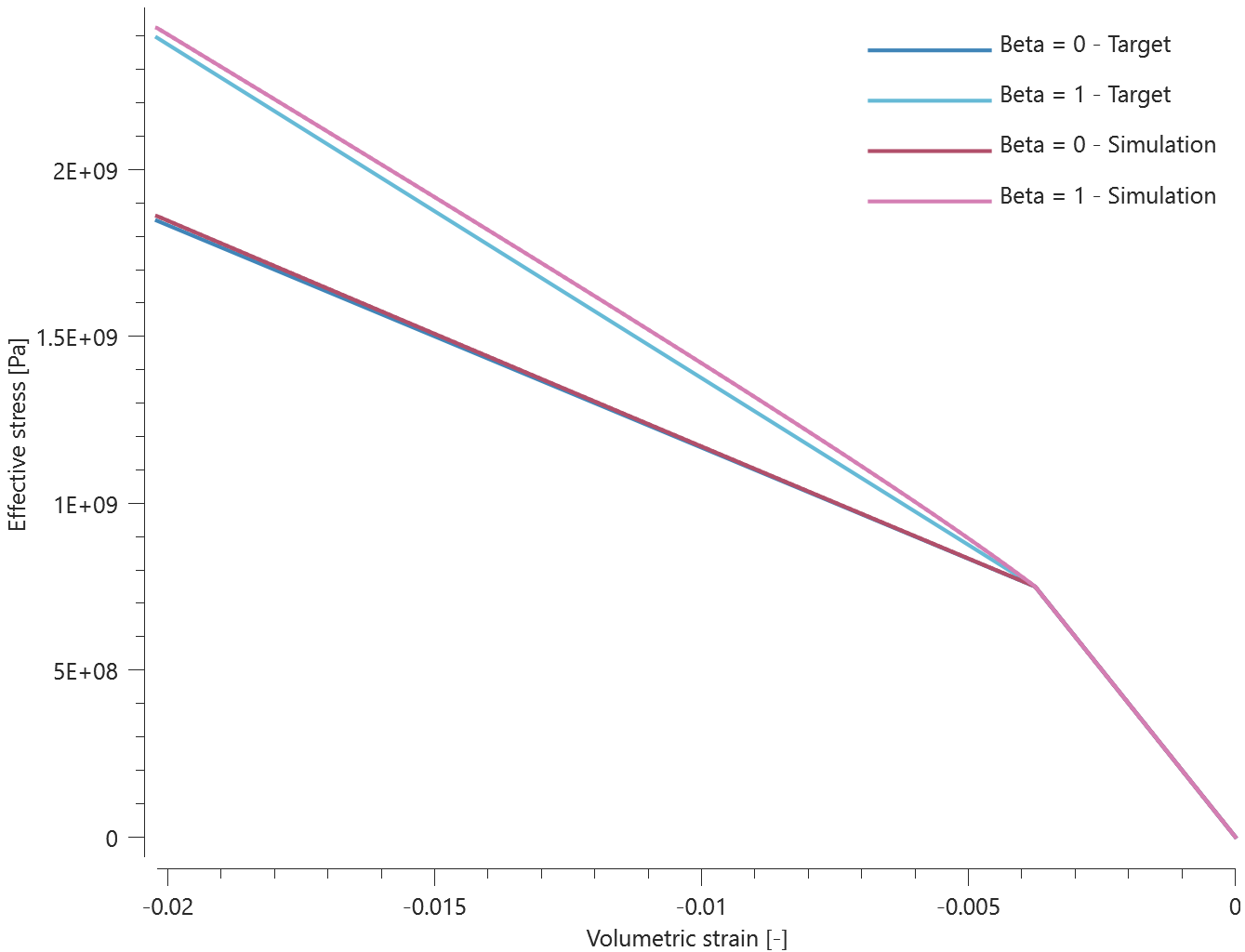
Last and average values of pressure, effective stress and volumetric strain are checked in the elements.
Tests
This benchmark is associated with 1 tests.
Pressure-volume relationship
"Optional title"
mid, $\rho$, $G$
$A_0$, $B_0$, $A_f$, $B_f$, $\varepsilon_f$, $\sigma_s$, $t_s$, $\alpha_s$
$K_1$, $K_2$, $K_3$, $\beta$, $K_c$, $\sigma_0^{max}$, $\sigma_f^{max}$
The pressure-volume relationship in *MAT_CERAMIC is verified in this test.
Tested parameters: $G$, $K_1$, $K_2$ and $K_3$.
The model consist of two CHEX elements. One of the elements is stretched and the other is compressed. Pressure vs. volumetric strain from the elements are presented in Figure 1 and 2 together with target curves from a verification script.
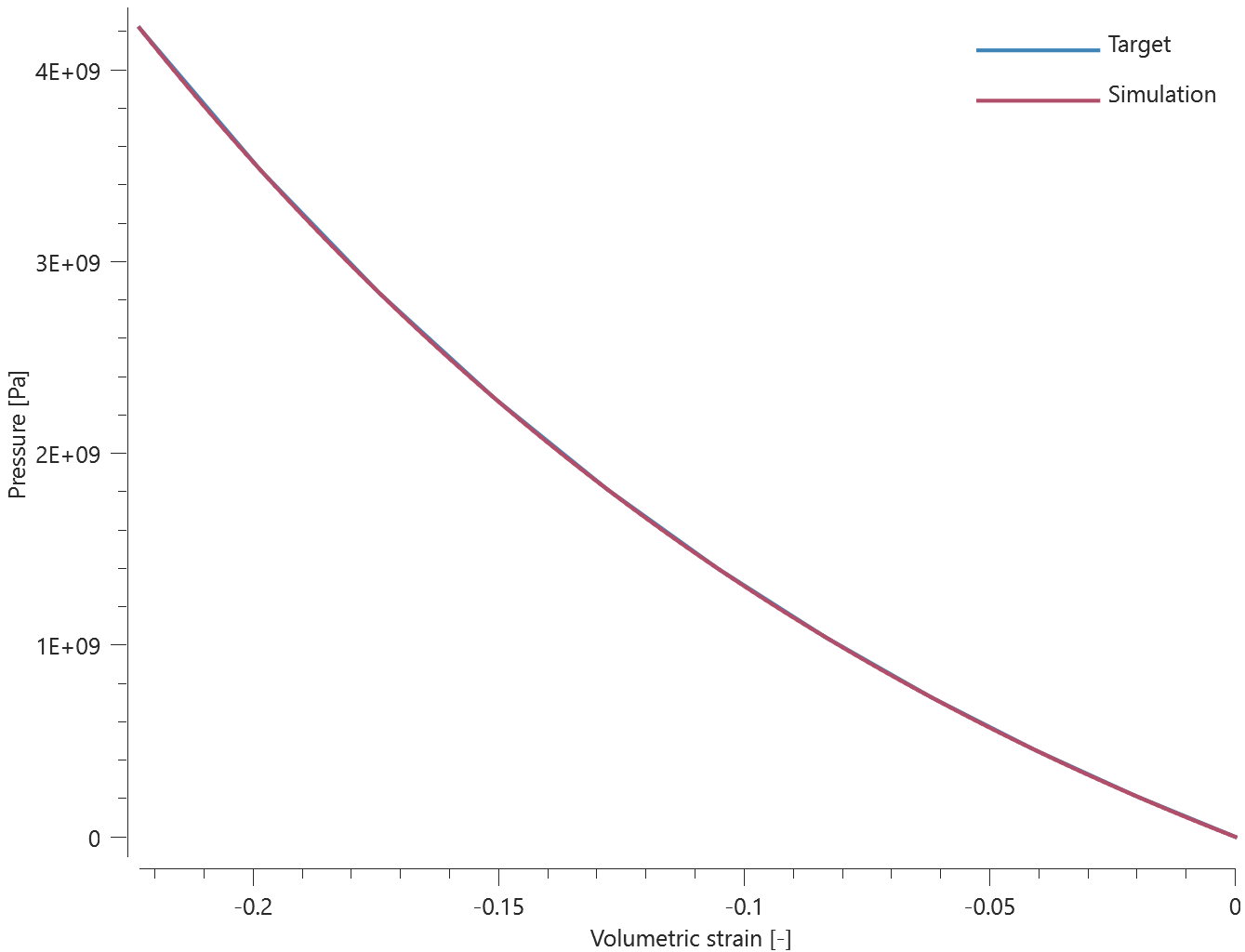
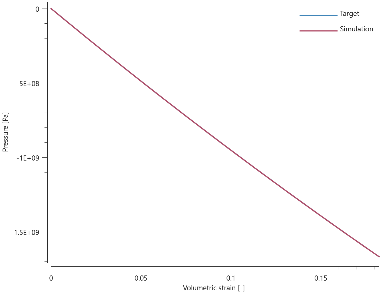
Maximum, minimum and average pressure are checked in the elements.
Tests
This benchmark is associated with 1 tests.
Spalling damage
"Optional title"
mid, $\rho$, $G$
$A_0$, $B_0$, $A_f$, $B_f$, $\varepsilon_f$, $\sigma_s$, $t_s$, $\alpha_s$
$K_1$, $K_2$, $K_3$, $\beta$, $K_c$, $\sigma_0^{max}$, $\sigma_f^{max}$
Spalling damage in *MAT_CERAMIC is verified in this test.
Tested parameters: $\sigma_s$, $t_s$ and $\alpha_s$.
A CHEX element is loaded in uniaxial tension. The element is stretched to a target stress and then kept at this stress level throughout the simulation. The target stress is greater than the defined spalling stress, meaning that damage starts to develop.
The time, $t$, at which failure should occur is calculated as:
$$ t = \frac{t_s}{\left(\sigma_1/\sigma_s\right)^{\alpha_s}} $$
Time $t$ is used as termination time in the simulation. Damage vs. time from the element is displayed in Figure 1 together with a target curve.
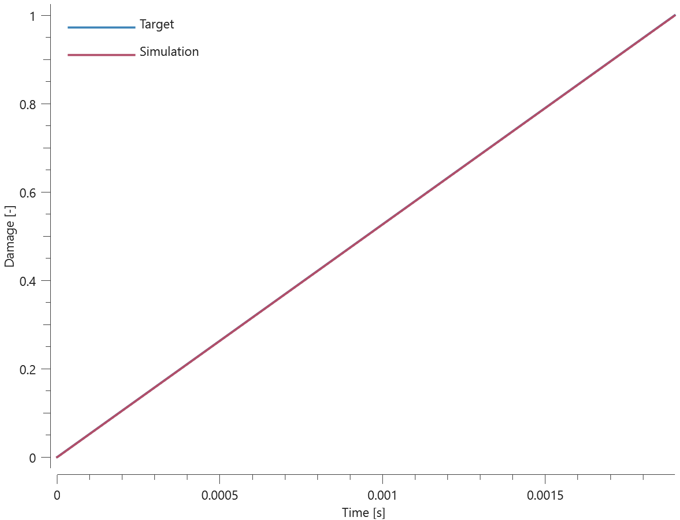
Maximum and average damage are checked.
Tests
This benchmark is associated with 1 tests.
Yield and failure surface
"Optional title"
mid, $\rho$, $G$
$A_0$, $B_0$, $A_f$, $B_f$, $\varepsilon_f$, $\sigma_s$, $t_s$, $\alpha_s$
$K_1$, $K_2$, $K_3$, $\beta$, $K_c$, $\sigma_0^{max}$, $\sigma_f^{max}$
The yield surface and failure surface in *MAT_CERAMIC are verified in this test.
Tested parameters: $A_0$, $B_0$, $\sigma_0^{max}$, $A_f$, $B_f$, $\sigma_f^{max}$ and $\varepsilon_f$.
Four CHEX elements are used in this test, which is divided into two steps.
In step 1, two of the elements are loaded to confinement pressures P3 and P4.
In step 2, one of the elements is stretched while the others are compressed.
The loading continues until failure occurs in all elements. With the selected crushing strain, failure occurs as soon as the effective stress reaches the yield surface. The loading conditions for each of the elements are presented in Table 1.
| Element ID | Step 1, Confinement pressure | Step 2, Loading |
|---|---|---|
| 1 | 0 | tension |
| 2 | 0 | compression |
| 3 | P3 | compression |
| 4 | P4 | compression |
Effective stress vs. pressure prior to and post failure in the elements are presented in Figure 1 together with the defined yield surface and failure surface.
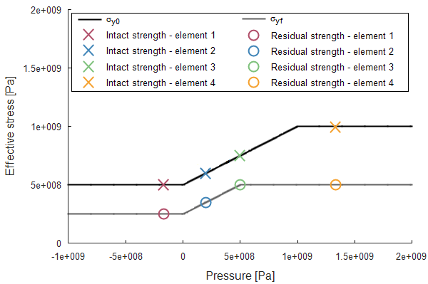
Note that each loading case is based on a singe element. If several elements were to be used in the specimen loaded in tension, node splitting would occur and the strength post failure would be zero.
Maximum, minimum and average effective stress are checked in the elements.
Tests
This benchmark is associated with 2 tests.
*MAT_CONCRETE_2018
Compaction curve
"Optional title"
mid, $\rho$, $G$
$K_0$, $K_L$, $p_0$, $p_L$, $\varepsilon_L$, $n$, $f_t$, $f_c$
$r_f$, $r_e$, $\varepsilon_t$, $\varepsilon_c$, $c$, $c_{dec}$, $\xi$, bulk
$K_{Ic}$
The compaction curve (pressure vs. inelastic volumetric strain) in *MAT_CONCRETE_2018 is verified in this test.
Tested parameters: $K_0$, $K_L$, $P_0$, $P_L$ and $\varepsilon_L$.
A CHEX element is volumetrically compressed. The pressure vs. volumetric strain repsonse is linear up to the crush limit, $P_0$, and defined by the bulk modulus, $K_0$. A quadratic response as a function of the volumetric plastic strain is then assumed until the material is fully compacted, which is defined by $P_L$ and $\varepsilon_L$. With further compaction, the response is linear and defined by the bulk modulus $K_L$.
Pressure vs. volumetric strain from the simulation is displayed in Figure 1 together with a target curve from a verification script.
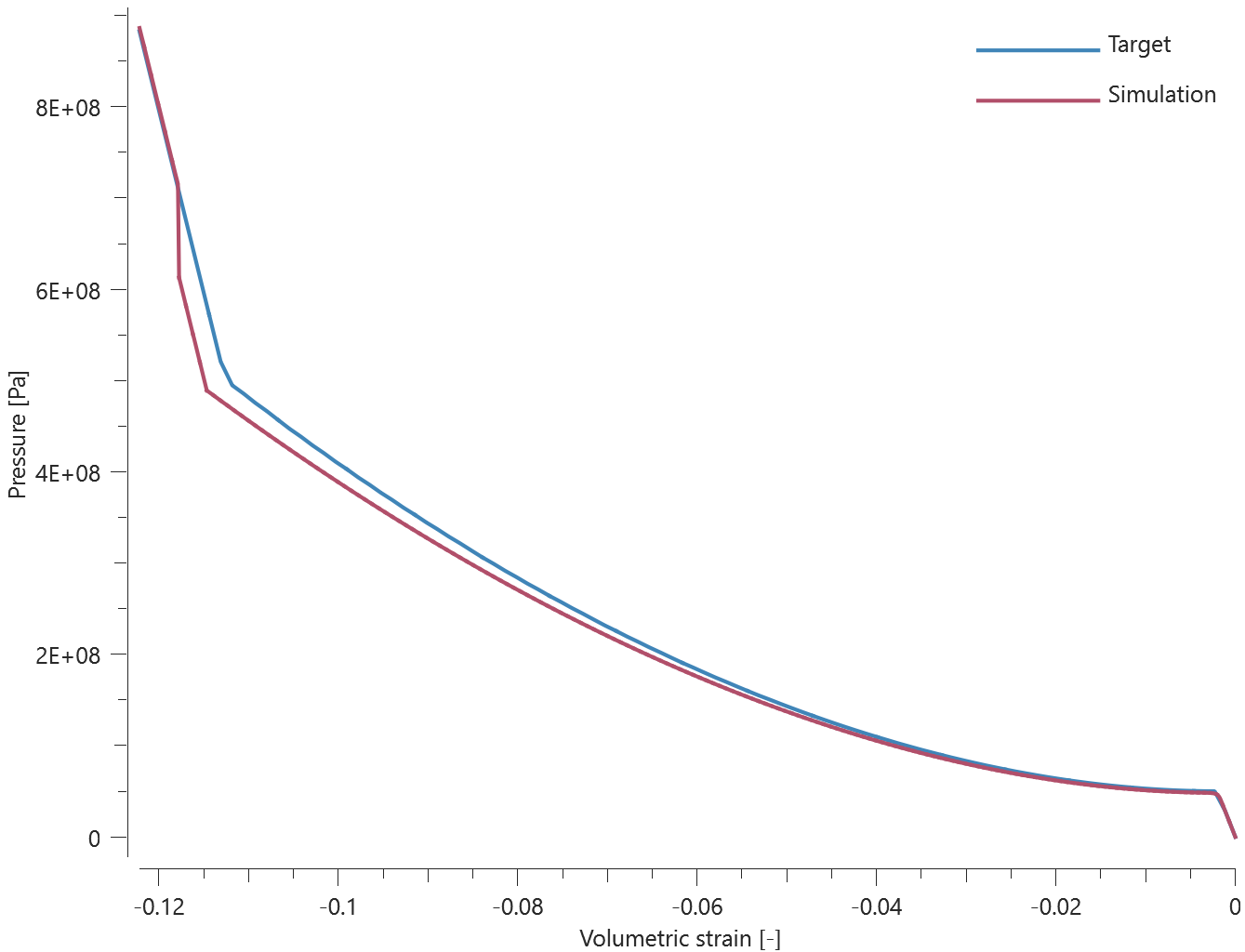
Maximum and average pressure are checked.
Tests
This benchmark is associated with 1 tests.
Crushing damage
"Optional title"
mid, $\rho$, $G$
$K_0$, $K_L$, $p_0$, $p_L$, $\varepsilon_L$, $n$, $f_t$, $f_c$
$r_f$, $r_e$, $\varepsilon_t$, $\varepsilon_c$, $c$, $c_{dec}$, $\xi$, bulk
$K_{Ic}$
Crushing damage in *MAT_CONCRETE_2018 is verified in this test.
Tested parameters: $K_0$, $K_L$, $P_0$, $P_L$, $\varepsilon_L$, $n$ and $\varepsilon_c$.
A CHEX element is loaded in uniaxial compression until failure occurs. Crushing damage vs. effective plastic strain from the element is displayed in Figure 1 together with a target curve from a verification script.
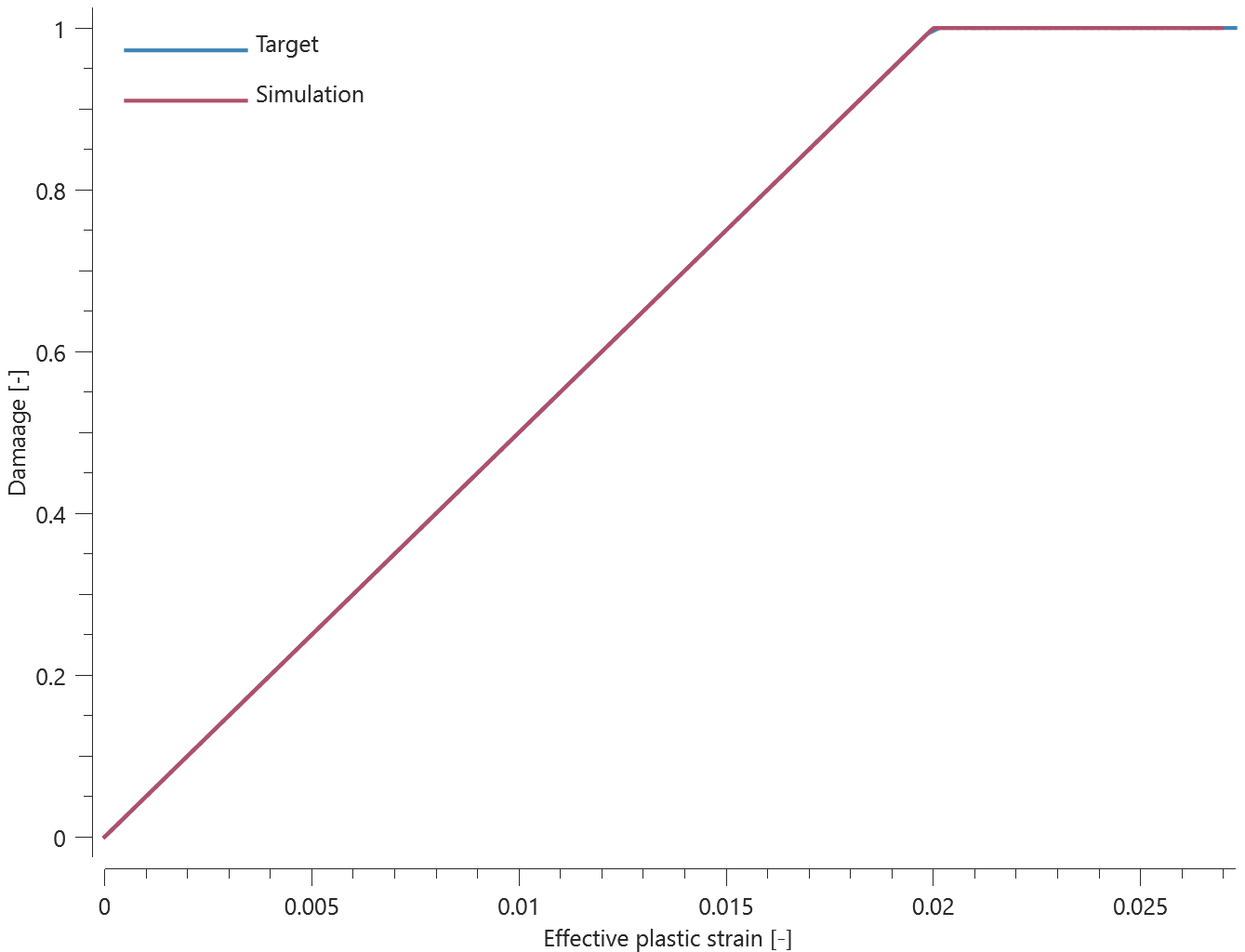
Maximum and average damage and effective plastic strain are checked.
Tests
This benchmark is associated with 1 tests.
Uniaxial tests
"Optional title"
mid, $\rho$, $G$
$K_0$, $K_L$, $p_0$, $p_L$, $\varepsilon_L$, $n$, $f_t$, $f_c$
$r_f$, $r_e$, $\varepsilon_t$, $\varepsilon_c$, $c$, $c_{dec}$, $\xi$, bulk
$K_{Ic}$
This deviatoric yield surface in *MAT_CONCRETE_2018 is verified in this test.
Tested parameters: $f_t$ and $f_c$.
The model consist of two CHEX elements. One of the elements is loaded in uniaxial compression and the other in uniaxial tension. The compressive strength is set to $50 \ MPa$ and the tensile strength to $5 \ MPa$.
Effective stress vs. time from both elements are presented in Figure 1 together with targets of the compressive and tensile strength.
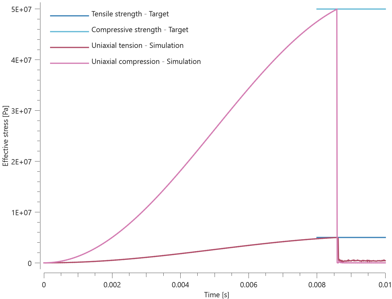
Maximum and average effective stress are checked in the elements.
Tests
This benchmark is associated with 1 tests.
Viscous damping
"Optional title"
mid, $\rho$, $G$
$K_0$, $K_L$, $p_0$, $p_L$, $\varepsilon_L$, $n$, $f_t$, $f_c$
$r_f$, $r_e$, $\varepsilon_t$, $\varepsilon_c$, $c$, $c_{dec}$, $\xi$, bulk
$K_{Ic}$
Viscous damping in *MAT_CONCRETE_2018 is verified in this test.
Tested parameters: $c$ and $c_{dec}$.
Two CHEX elements are loaded in uniaxial compression. The compression is done at a prescribed strain rate and damping is used in one of the elements. Effective stress vs. time from the elements are presented in Figure 1 together with target curves from a verification script.
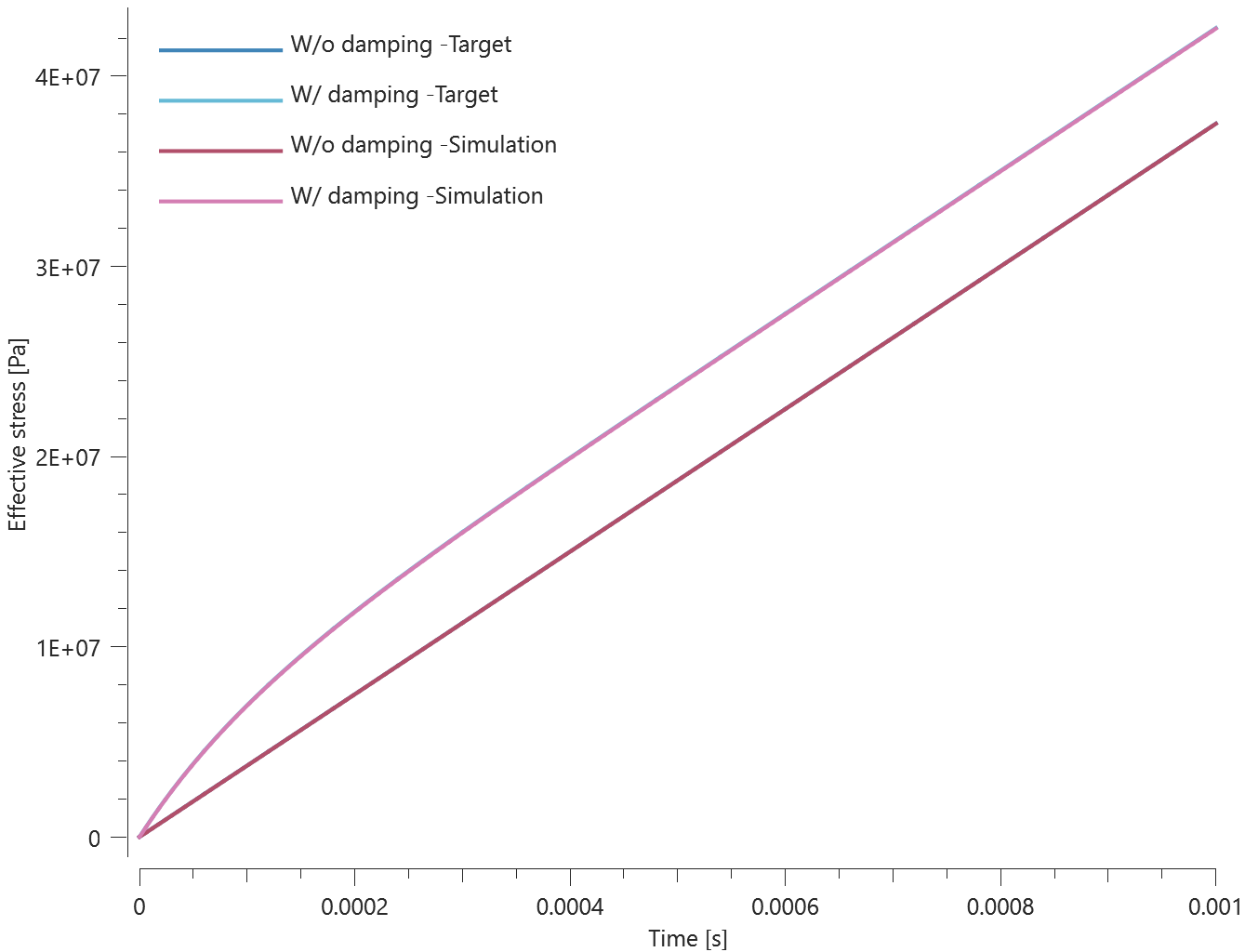
Maximum and average effective stress are checked in the elements.
Tests
This benchmark is associated with 1 tests.
*MAT_CREEP
Elastoplasticity
"Optional title"
mid, $\rho$, $E$, $\nu$, did, tid
$A$, $B$, $n$, $c_0$, $c_1$, $c_2$, $c_3$
The elasto-plastic response in *MAT_CREEP is verified in this test.
Tested parameters: $E$, $A$, $B$ and $n$.
A CHEX element is stretched in the X-direction while fixed in the Y- and Z-direction. Effective stress vs. volumetric strain from the element is displayed in Figure 1 together with a target curve obtained from a verification script.
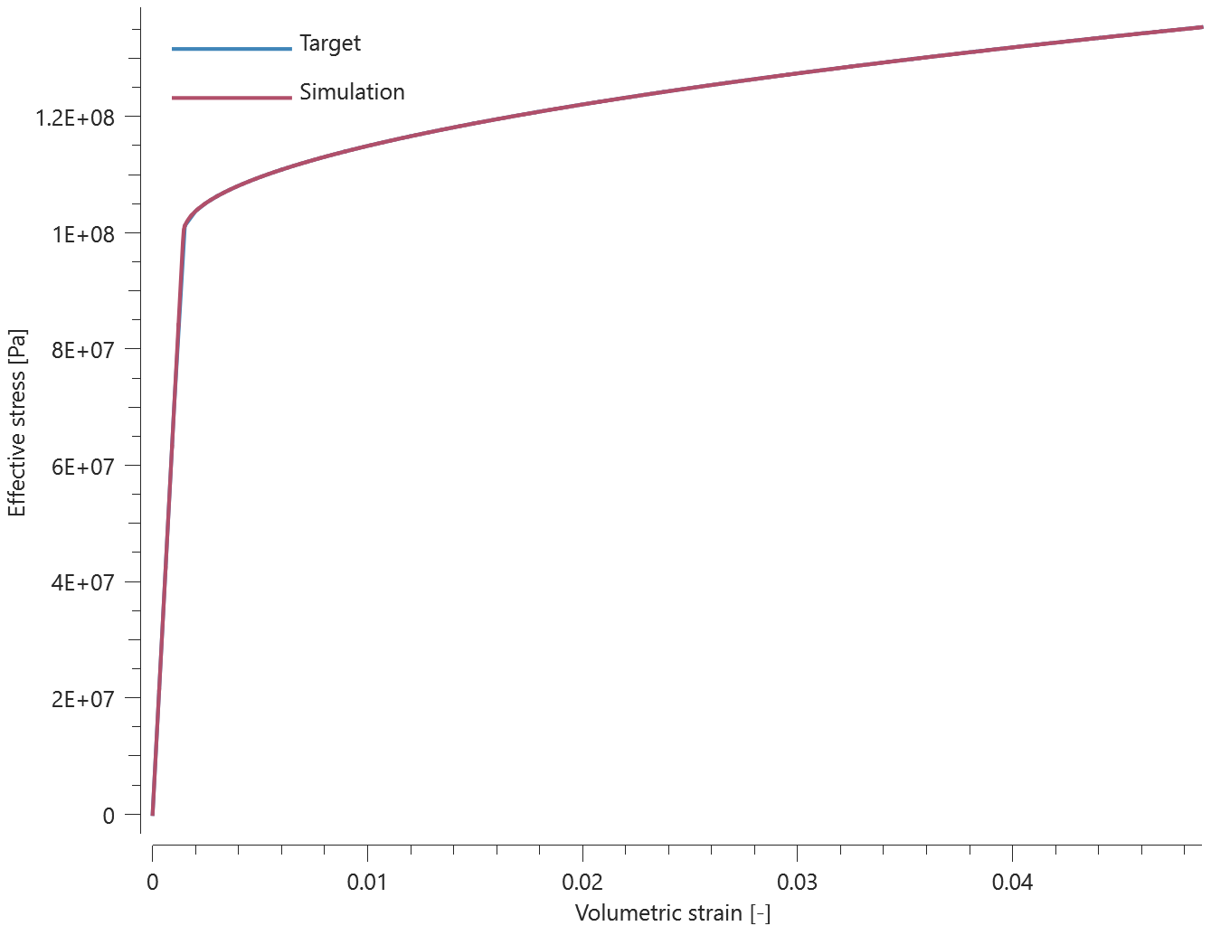
Maximum and average effective stress and volumetric strain are checked.
Tests
This benchmark is associated with 1 tests.
Viscoelasticity
"Optional title"
mid, $\rho$, $E$, $\nu$, did, tid
$A$, $B$, $n$, $c_0$, $c_1$, $c_2$, $c_3$
The visco-elastic response in *MAT_CREEP is verified in this test.
Tested paramters: $E$, $c_0$, $c_1$, $c_2$ and $c_3$.
A CHEX element is loaded in uniaxial tension. The viscous parameters $c_0$ and $c_1$ are defined as constants while $c_2$ is defined by a function and $c_3$ by a curve. The viscous parameters are selected so that they all have a significant effect on the stress. Temperature is prescribed as a function of time.
Effective stress vs. effective creep strain from the element is presented in Figure 1 together with a target curve obtained from a verification script.
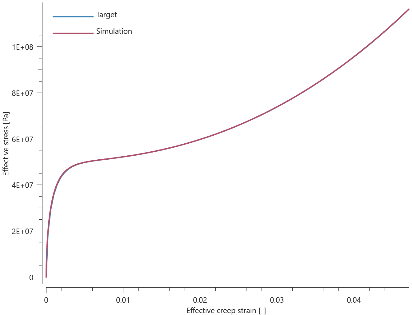
Maximum and average effective stress and effective creep strain are checked.
Tests
This benchmark is associated with 1 tests.
*MAT_ELASTIC
Linear elasticity
"Optional title"
mid, $\rho$, $E$, $\nu$, did, tid
$a$, $b$, $c$, $c_{dec}$
Linear elasticity in *MAT_ELASTIC is verified in this test.
Tested parameters: $E$ and $\nu$.
A CHEX element is stretched in the X-direction while fixed in the Y- and Z-direction. Stress in X-, Y- and Z-direction vs. volumetric strain from the element are presented in Figure 1 together with target curves from a verification script.
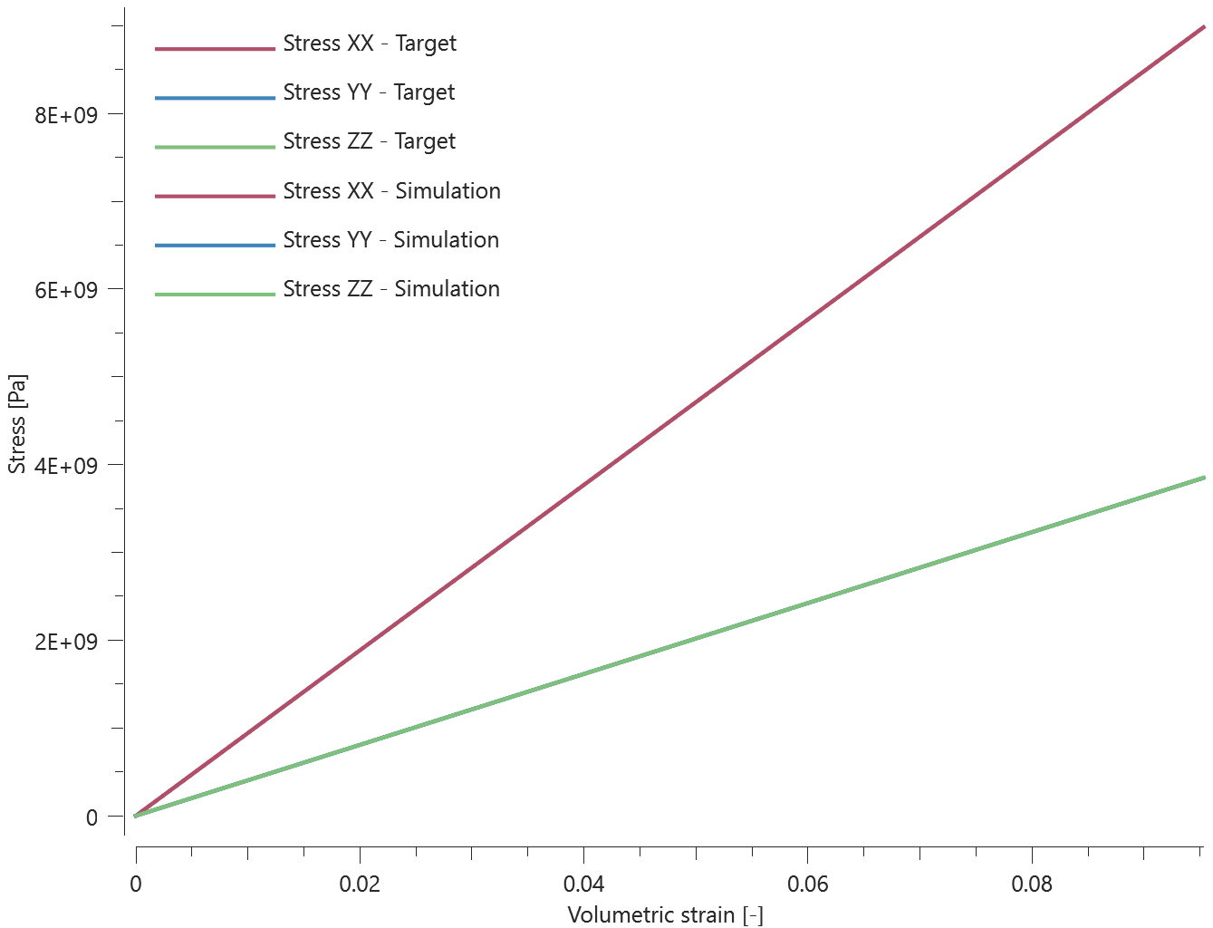
Maximum and average volumetric strain and stress in X-, Y- and Z-direction are checked.
Tests
This benchmark is associated with 1 tests.
Non-linear elasticity
"Optional title"
mid, $\rho$, $E$, $\nu$, did, tid
$a$, $b$, $c$, $c_{dec}$
Non-linear elasticity in *MAT_ELASTIC is verified in this test.
Tested parameters: $E$, $\nu$, $A$ and $B$.
A CHEX element is stretched in the X-direction while fixed in the Y- and Z-direction. Stress in X-, Y- and Z-direction vs. volumetric strain from the element are presented in Figure 1 together with target curves from a verification script.
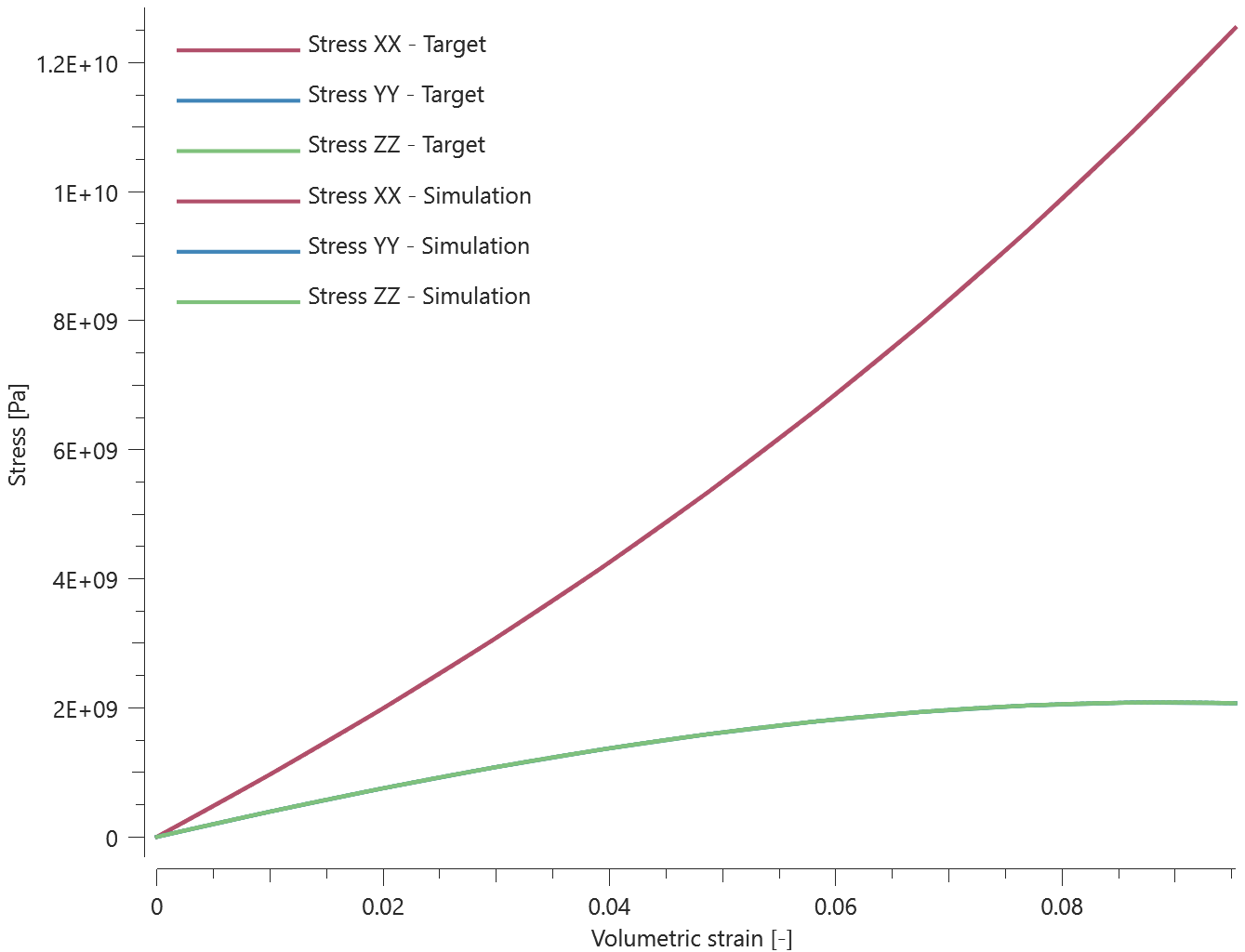
Maximum and average volumetric strain and stress in X-, Y- and Z-direction are checked.
Tests
This benchmark is associated with 1 tests.
Non-linear elasticity with damping
"Optional title"
mid, $\rho$, $E$, $\nu$, did, tid
$a$, $b$, $c$, $c_{dec}$
Non-linear elasticity with damping in *MAT_ELASTIC is verified in this test.
Tested parameters: $E$, $\nu$, $a$, $b$, $c$ and $c_{dec}$.
A CHEX element is stretched in the X-direction while fixed in the Y- and Z-direction. Stress in X-, Y- and Z-direction vs. volumetric strain from the element are presented in Figure 1 together with target curves from verification script.
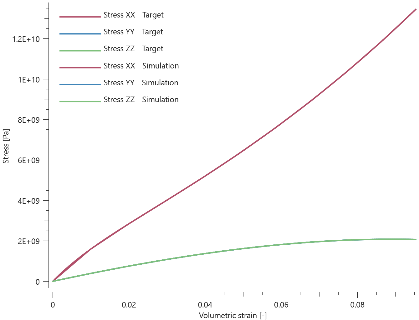
Maximum and average volumetric strain and stress in X-, Y- and Z-direction are checked.
Tests
This benchmark is associated with 1 tests.
*MAT_FABRIC
Dynamic viscocity
"Optional title"
mid, $\rho$, $E$, $\nu$
$E_f$, $\varepsilon_l$, $\varepsilon_{f0}$, $\varepsilon_{f1}$, $\varepsilon_e$, $\sigma_y$, $K_n$, $n$
$\alpha_1$, $\alpha_2$, $\alpha_3$, $\alpha_4$, $\eta_1$, $\eta_2$, $\eta_3$, $\eta_4$
$\mu$, $\xi$, $c$, $\dot{\varepsilon}_0$, $W_c$
The dynamic viscocity in *MAT_FABRIC is verified in this test.
Tested parameter: $\mu$.
Two CHEX elements are loaded in uniaxial compresssion. A dynamic viscosity is defined for one of the elements. Effective stress vs. time from both elements is presented in Figure 1 together with target curves obtained from, a verification script.
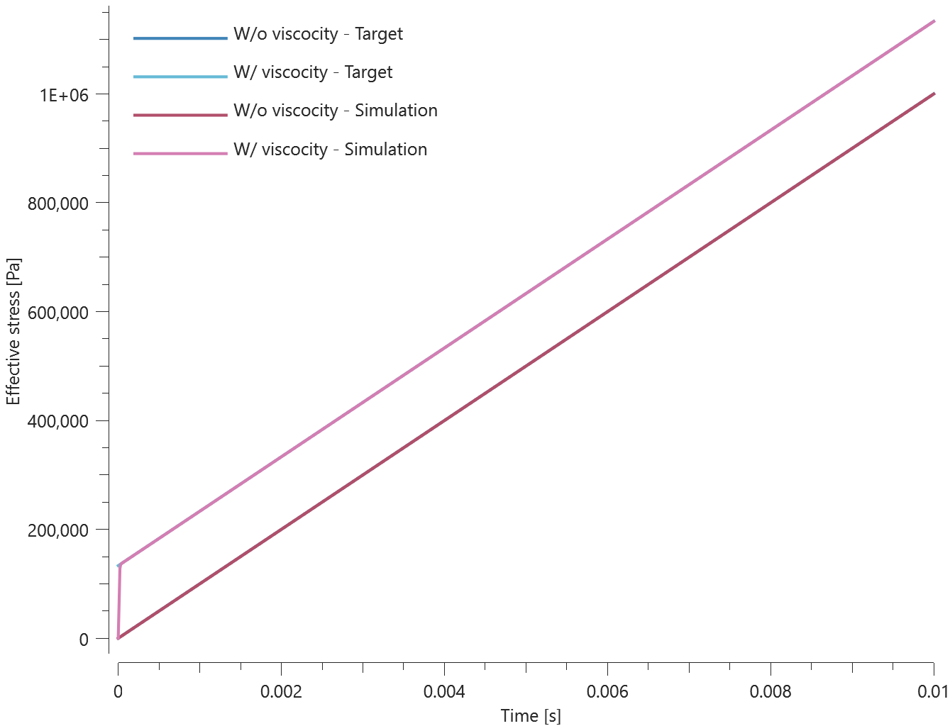
Maximum and average effective stress are checked in both elements.
Tests
This benchmark is associated with 1 tests.
Fiber properties
"Optional title"
mid, $\rho$, $E$, $\nu$
$E_f$, $\varepsilon_l$, $\varepsilon_{f0}$, $\varepsilon_{f1}$, $\varepsilon_e$, $\sigma_y$, $K_n$, $n$
$\alpha_1$, $\alpha_2$, $\alpha_3$, $\alpha_4$, $\eta_1$, $\eta_2$, $\eta_3$, $\eta_4$
$\mu$, $\xi$, $c$, $\dot{\varepsilon}_0$, $W_c$
The stiffness, locking strain and rate dependent failure strains of the fibers in *MAT_FABRIC are verified in this test.
Tested parameters: $E_f$, $\varepsilon_l$, $\varepsilon_{f0}$, $\varepsilon_{f1}$, $\alpha_1$ - $\alpha_4$, $\eta_1$ - $\eta_4$, $c$ and $\dot{\varepsilon}_0$.
Two CHEX elements with fibers defined in the X-direction are used in this test. One of the elements is loaded in uniaxial tension and the other in uniaxial compression. The loading occurs in the fiber direction. Deformations occur at a constant strain rate and the fiber failure strains are defined to be strain rate dependent.
Stress vs. strain in the fiber direction from both elements are presented in Figure 1 together with target curves obtained from a verification script.
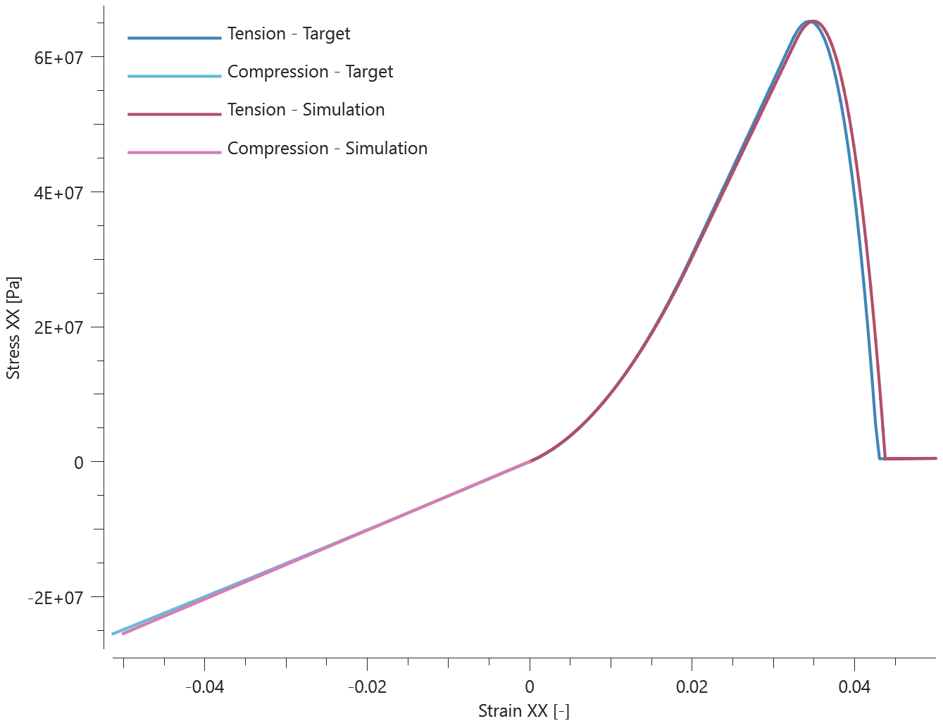
Maximum and average stress in the fiber direction are checked in both elements.
Tests
This benchmark is associated with 1 tests.
Matrix properties
"Optional title"
mid, $\rho$, $E$, $\nu$
$E_f$, $\varepsilon_l$, $\varepsilon_{f0}$, $\varepsilon_{f1}$, $\varepsilon_e$, $\sigma_y$, $K_n$, $n$
$\alpha_1$, $\alpha_2$, $\alpha_3$, $\alpha_4$, $\eta_1$, $\eta_2$, $\eta_3$, $\eta_4$
$\mu$, $\xi$, $c$, $\dot{\varepsilon}_0$, $W_c$
The stiffness, yield strength and failure of the matrix in *MAT_FABRIC are verified in this test.
Tested parameters: $E$, $\nu$, $\sigma_y$ and $W_c$.
A CHEX element without fibers is loaded in uniaxial tension until failure occurs. Stress vs. strain from the element is presented in Figure 1 together with a target curve from a verification script.
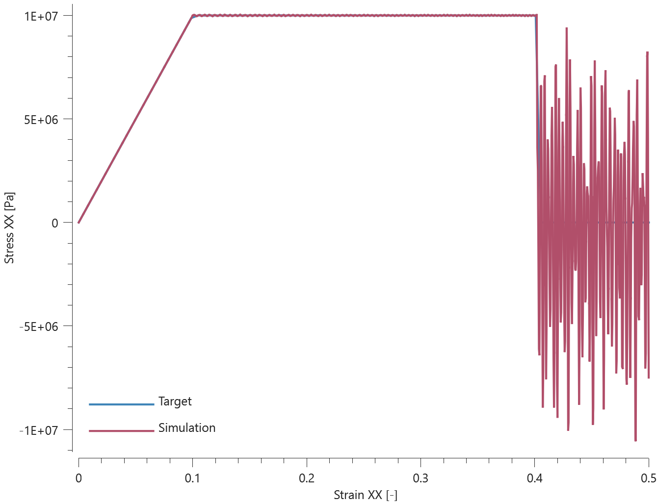
Maximum and average stress are checked.
Tests
This benchmark is associated with 1 tests.
Non-linear bulk stiffness
"Optional title"
mid, $\rho$, $E$, $\nu$
$E_f$, $\varepsilon_l$, $\varepsilon_{f0}$, $\varepsilon_{f1}$, $\varepsilon_e$, $\sigma_y$, $K_n$, $n$
$\alpha_1$, $\alpha_2$, $\alpha_3$, $\alpha_4$, $\eta_1$, $\eta_2$, $\eta_3$, $\eta_4$
$\mu$, $\xi$, $c$, $\dot{\varepsilon}_0$, $W_c$
The non-linear bulk stiffness in *MAT_FABRIC is verified in this test.
Tested parameters: $K_n$ and $n$.
Two CHEX elements are used in this test. The elements are being compressed in the Z-direction while fixed in the X- and Y-direction. A non-linear bulk stiffness is assumed in one of the elements. Pressure vs. volumetric strain from both elements are presented in Figure 1 together with target curves obtained from a verification script.
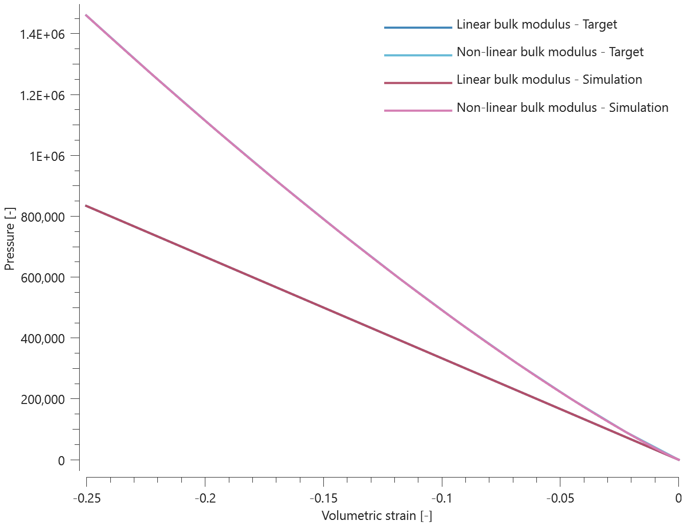
Maximum and average pressure are checked in both elements.
Tests
This benchmark is associated with 1 tests.
*MAT_FLUID
Pressure with cap
"Optional title"
mid, $\rho$, $K$, $\mu$, $p_c$, eosid
$G$
The consitutive relation for volumetric strains in *MAT_FLUID is verified in this test.
Tested parameters: $K$ and $p_c$.
Two CHEX elements are used in this test. One of the elements is volumetrically compressed while the other is volumetrically expanded. A pressure cap is defined and it should only affect the expanding element.
Pressure vs. volumetric strain from both elements are presented in Figure 1 together with target curves from a verification script.
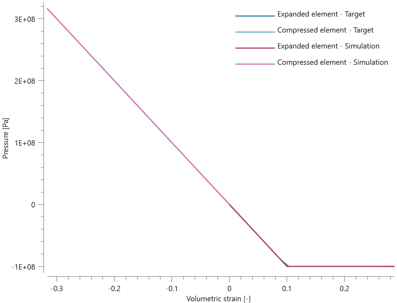
Maximum, minimum and average pressure are checked in the elements.
Tests
This benchmark is associated with 1 tests.
Shear resistance
"Optional title"
mid, $\rho$, $K$, $\mu$, $p_c$, eosid
$G$
The consititutive relation for deviatoric strains in *MAT_FLUID is verified in this test.
Tested parameters: $G$.
A CHEX element is sheared. The artificial shear modulus, $G$, is set to $1.5\cdot K$. The shear stress vs. time from the simulation is compared to a target curve in Figure 1.
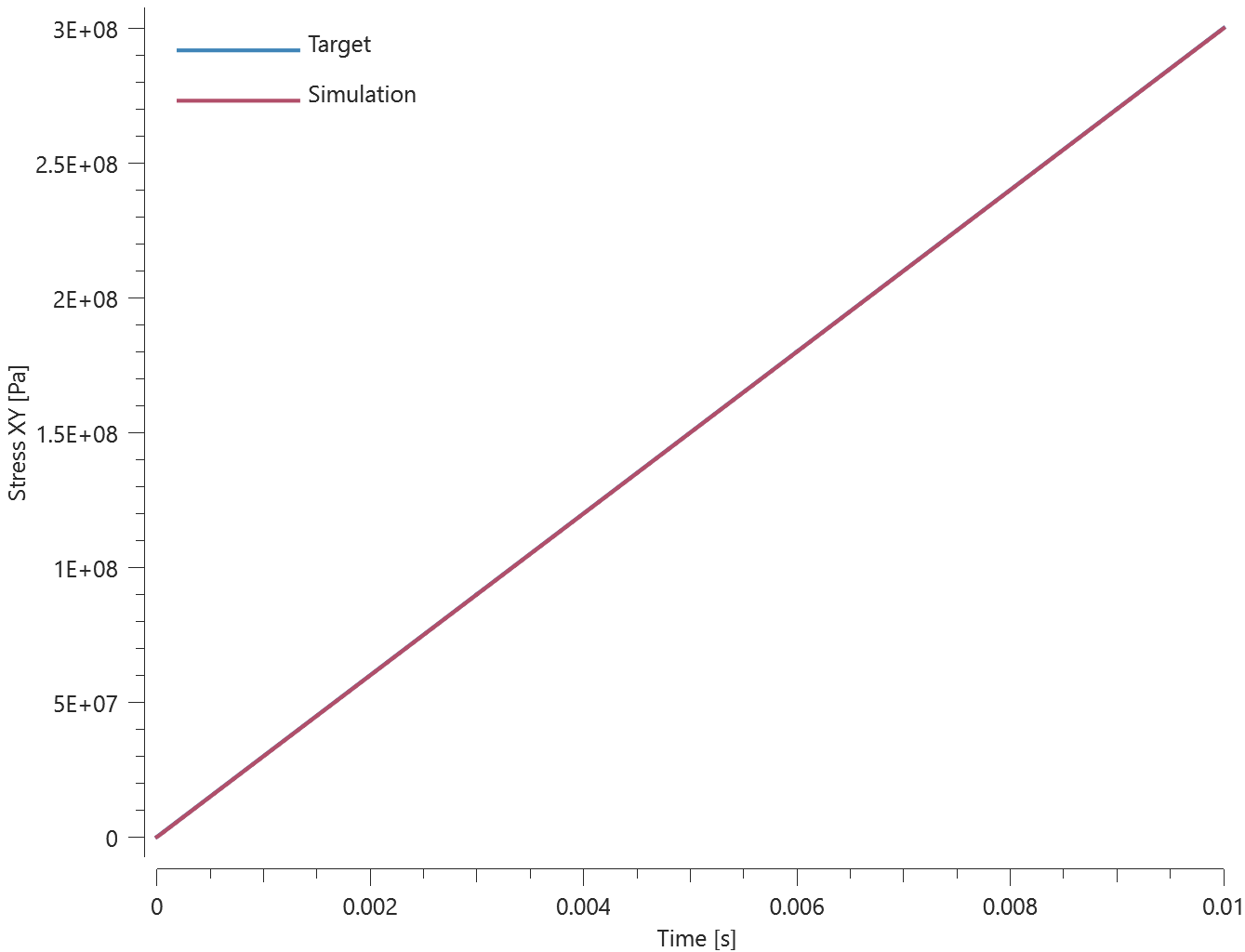
Maximum and average stress are checked.
Tests
This benchmark is associated with 1 tests.
*MAT_FOAM
Revision test
"Optional title"
mid, $\rho$, $E$, $\nu$, did
cid, $tsc$, $\beta$
This is a revision test for *MAT_FOAM.
Tested parameters: $\rho$, $E$, $\nu$, cid and $tsc$.
The reaction force in the Z-direction is checked.
Tests
This benchmark is associated with 1 tests.
*MAT_FORMING
Initial backstress
"Optional title"
mid, $\rho$, $E$, $\nu$, did, tid
cid, $\xi$, $a_0$, $a_1$
$\varepsilon_{1}$, $\varepsilon_{2}$, $\varepsilon_{3}$, $\sigma_{1}$, $\sigma_{2}$, $\sigma_{3}$
The initial back stress of *MAT_FORMING is verified in this test.
Tested parameters: $\sigma_{1}$, $\sigma_{2}$ and $\sigma_{3}$.
The intial backstress is entered as:
$$ \sigma_1 = \frac{2}{3}\sigma_0 $$
$$ \sigma_2 = \sigma_3 = -\frac{1}{3}\sigma_0 $$
The initial back stresses are checked.
Tests
This benchmark is associated with 1 tests.
Isotropic and kinematic hardening
"Optional title"
mid, $\rho$, $E$, $\nu$, did, tid
cid, $\xi$, $a_0$, $a_1$
$\varepsilon_{1}$, $\varepsilon_{2}$, $\varepsilon_{3}$, $\sigma_{1}$, $\sigma_{2}$, $\sigma_{3}$
The isotropic and kinematic hardening in *MAT_FORMING are verified in this test.
Tested parameters: $E$, cid and $\xi$.
Two CHEX elements are subjected to a cyclic uniaxial load. Isotropic hardening is used in one of the elements and kinematic hardening in the other. Stress vs. time from the elements are presented in Figure 1 and 2 together with target curves from a verification script.
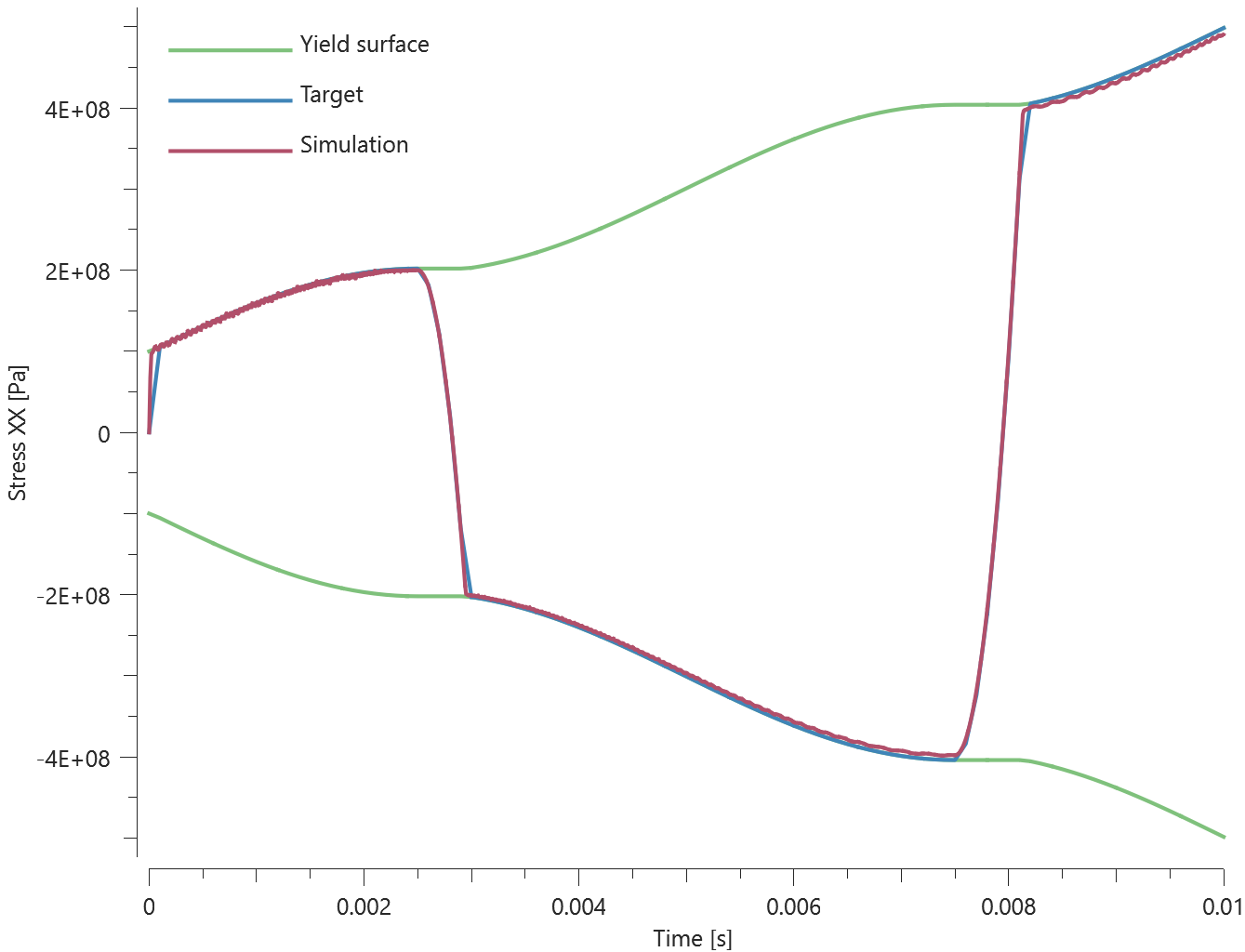
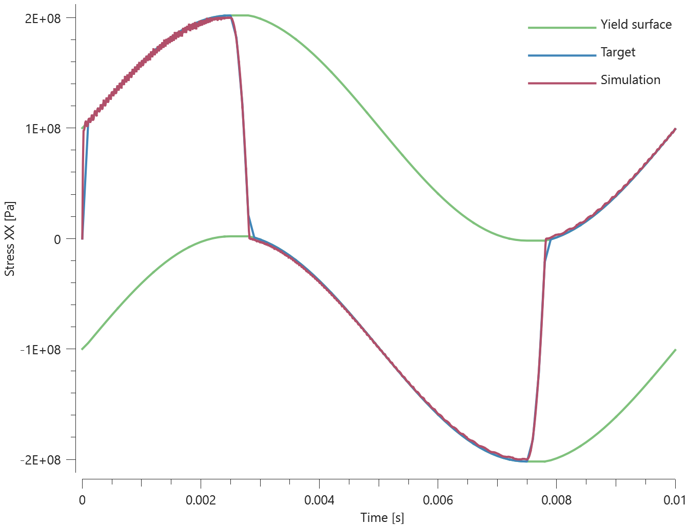
Maximum, minimum and average stress in the loading direction are checked in the elements.
Tests
This benchmark is associated with 1 tests.
*MAT_FORMING_R
Damage softening
"Optional title"
mid, $\rho$, $E$, $\nu$, did, tid
cid, $\xi$, $R_{00}$, $R_{45}$, $R_{90}$, $s_0$, $s_1$
Damage softening in *MAT_FORMING_R is verified in this test.
Tested parameters: $s_0$ and $s_1$.
Two CHEX elements are loaded in uniaxial tension until failure occurs. Parameters for failure are defined in *PROP_DAMAGE_CL.
Damage softening is defined for one of the elements. Effective stress vs. effective plastic strain from both elements are presented in Figure 1 together with target curves from a verification script.
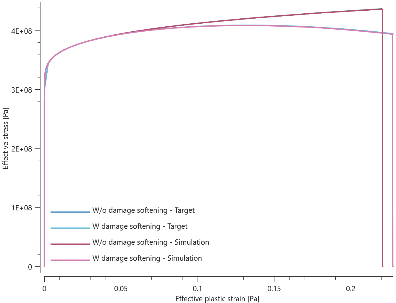
Maximum and average effective stress and effective plastic strain are checked in the elements.
Tests
This benchmark is associated with 1 tests.
Isotropic and kinematic hardening
"Optional title"
mid, $\rho$, $E$, $\nu$, did, tid
cid, $\xi$, $R_{00}$, $R_{45}$, $R_{90}$, $s_0$, $s_1$
The isotropic and kinematic hardening in *MAT_FORMING_R are verified in this test.
Tested parameters: $E$, cid and $\xi$.
Two CHEX elements are subjected to a cyclic uniaxial load. Isotropic hardening is used in one of the elements and kinematic hardening in the other. Stress vs. time from the elements are presented in Figure 1 and 2 together with target curves from a verification script.
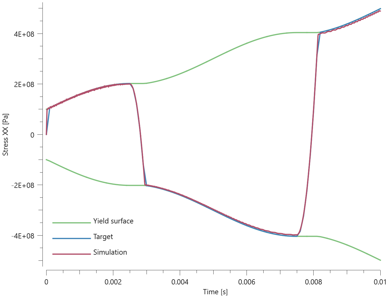
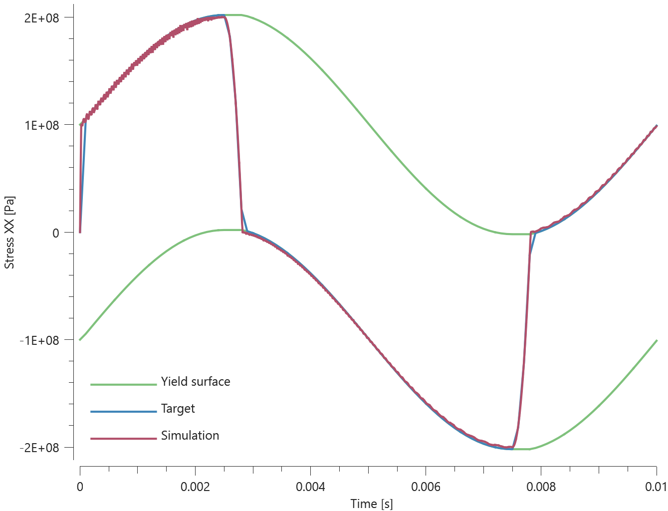
Maximum, minimum and average stress in the loading direction are checked in the elements.
Tests
This benchmark is associated with 1 tests.
R-values
"Optional title"
mid, $\rho$, $E$, $\nu$, did, tid
cid, $\xi$, $R_{00}$, $R_{45}$, $R_{90}$, $s_0$, $s_1$
The Lankford coefficients (R-values) of *MAT_FORMING_R are verified in this test.
Three CHEX elements are stretched in the global X-direction. Local coordinate systems are defined for each element. The local x- and y-direction expressed in the global coordiante system are presented in Table 1.
| Element ID | Local x-dir. [X,Y,Z] | Local y-dir. [X,Y,Z] |
|---|---|---|
| 1 | [$1, \ 0, \ 0$] | [$0, \ 1, \ 0$] |
| 2 | [$1/\sqrt{2}, \ 1/\sqrt{2}, \ 0$] | [$-1/\sqrt{2}, \ 1/\sqrt{2}, \ 0$] |
| 3 | [$0, \ 1, \ 0$] | [$-1, \ 0, \ 0$] |
Given the R-values and the strain in the X-direction at termination, the strain in the Y-direction at termination is calculated as:
Element 1: $$ \varepsilon_{yy} = - \varepsilon_{xx}/(1 + 1/R_{00}) $$
Element 2: $$ \varepsilon_{yy} = - \varepsilon_{xx}/(1 + 1/R_{45}) $$
Element 3: $$ \varepsilon_{yy} = - \varepsilon_{xx}/(1 + 1/R_{90}) $$
Last values of strain in Y-direction are checked in the elements.
Tests
This benchmark is associated with 1 tests.
*MAT_GRANULAR_CAP
Compaction curve
"Optional title"
mid, $\rho$, $E$, $\nu$
cid${}_1$, cid${}_2$, $\xi$, $\eta$, $\sigma_{dev}^{max}$, $B_0$, $B_1$
The compaction curve (pressure vs. inelastic volumetric strain) in *MAT_GRANULAR_CAP is verified in this test.
Tested parameters: $E$, $\nu$ and cid${}_1$.
A cubic box is compacted to a specified volumetric strain. Pressure vs. volumetric strain is presented in Figure 1 together with a target curve from a verification script. The test is done twice, once with the box as a CHEX element and once with the box built of SPH particles.
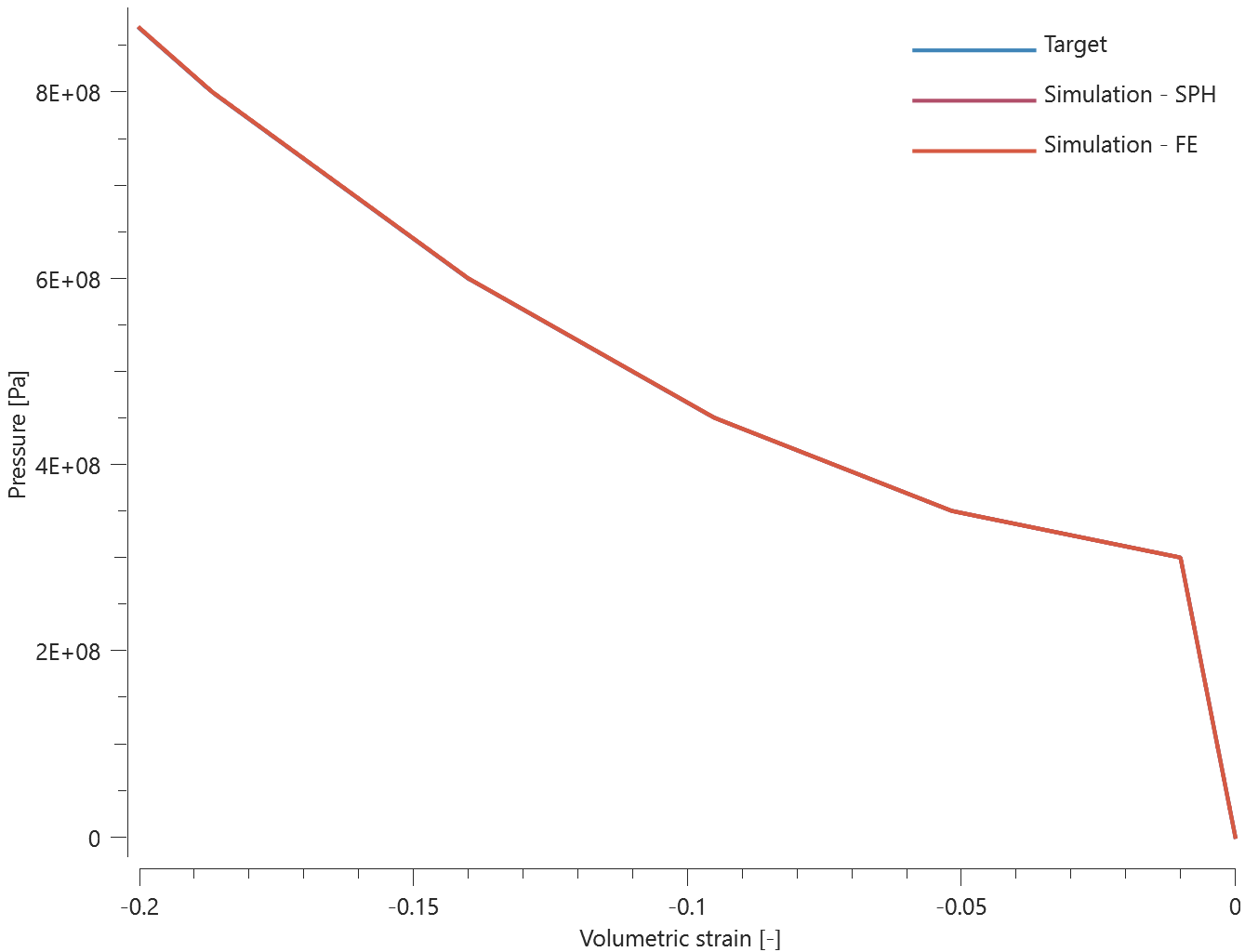
Maximum and average pressure and minimum and average volumetric strain are checked.
Tests
This benchmark is associated with 2 tests.
Damage
"Optional title"
mid, $\rho$, $E$, $\nu$
cid${}_1$, cid${}_2$, $\xi$, $\eta$, $\sigma_{dev}^{max}$, $B_0$, $B_1$
Damage caused by inelastic deviatoric deformations in *MAT_GRANULAR_CAP is verified in this test.
Tested parameters: $B_0$ and $B_1$.
Two cubix boxes are used in this test. One is loaded in uniaxial compression and the other in uniaxial tension. Damage vs. time from the elements are presented in Figure 1 together with target curves from a verification script. The test is done twice, once with the box as CHEX elements and once with the box built of SPH particles.
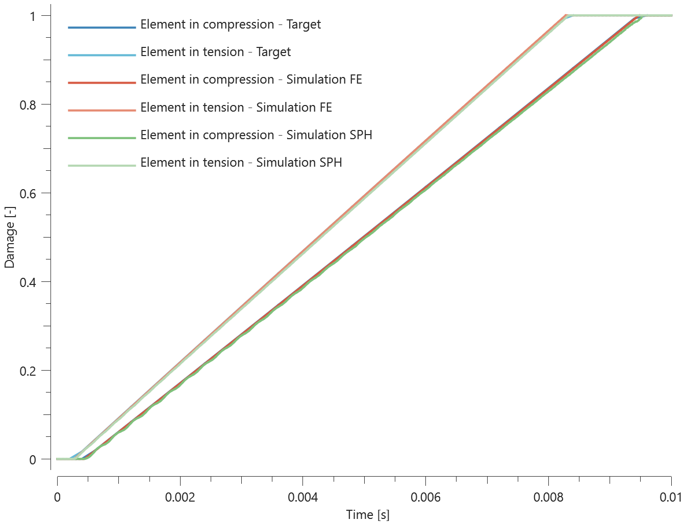
Maximum and average damage are checked in the elements.
Tests
This benchmark is associated with 2 tests.
Damage (cut-off criterion)
"Optional title"
mid, $\rho$, $E$, $\nu$
cid${}_1$, cid${}_2$, $\xi$, $\eta$, $\sigma_{dev}^{max}$, $B_0$, $B_1$
The damage cut-off criterion in *MAT_GRANULAR_CAP is verified in this test.
Tested parameters: $E$, $\nu$ and cid${}_2$.
A cubic box is volumetrically expanded until failure occurs. $cid_2/\sigma_a$ is defined as pressure independent and therefore failure should occur once the pressure reaches $-\sigma_a$. The test is done twice, once with the box as a CHEX element once with the box built of SPH particles.
The volumetric strain at failure, $\varepsilon_v$, is calculated as:
$$ \varepsilon_v = \sigma_a/K $$
The bulk modulus, $K$, is calculated as:
$$ K = \frac{E}{3(1-2\nu)} $$
The pressure is set to zero once the material fails. Pressure vs. volumetric strain in the element is compared to the target curve in Figure 1.
/mat_granular_cap_damage_cut-off_criterion_FE_SPH.png)
Minimum and average pressure and maximum and average volumetric strain are checked.
Tests
This benchmark is associated with 2 tests.
Yield surface
"Optional title"
mid, $\rho$, $E$, $\nu$
cid${}_1$, cid${}_2$, $\xi$, $\eta$, $\sigma_{dev}^{max}$, $B_0$, $B_1$
The deviatoric yield surface of *MAT_GRANULAR_CAP is verified in this test.
Tested parameters: $E$, $\nu$, $cid_1$, $cid_2$, $\eta$ and $\sigma_{dev}^{max}$.
Three cubic boxes are used in this test. Two of the elements are loaded in uniaxial compression while the third is loaded in uniaxial tension. For one of the elements in compression, a cap on the deviatoric yield stress is used. The adhesion stress is defined as pressure independent. The test is done twice, once with the boxes as a CHEX element once with the boxes built of SPH particles.
The volumetric strain, $\varepsilon_v$, pressure, $P$, and effective stress, $\sigma_{eff}$, once the yield surface is reached is calculated as follows.
Element in compression, without cap:
$$ \varepsilon_v = \sigma_a/ (\eta K - 3K) $$
$$ P = -K \varepsilon_v $$
$$ \sigma_{eff} = \eta (-K \varepsilon_v) + \sigma_a $$
Element in compression, with cap:
$$ \sigma_{eff} = min(\sigma_{dev}^{max}, \eta (-K \varepsilon_v)) + \sigma_a $$
$$ P = \sigma_{eff}/3 $$
$$ \varepsilon_v = -P/K $$
Element in tension:
$$ \varepsilon_v = \sigma_a/4K $$
$$ P = -K\varepsilon_v $$
$$ \sigma_{eff} = -K\varepsilon_v + \sigma_a $$
Note that the cap on the deviatoric yield stress only operates on the term $\eta \cdot p_c(\varepsilon_{vol}^{eff})$.
Effective stress vs. volumetric strain and pressure vs. volumetric strain from the CHEX elements are presented in Figure 1 and 2 together with targets based on the calculations above.
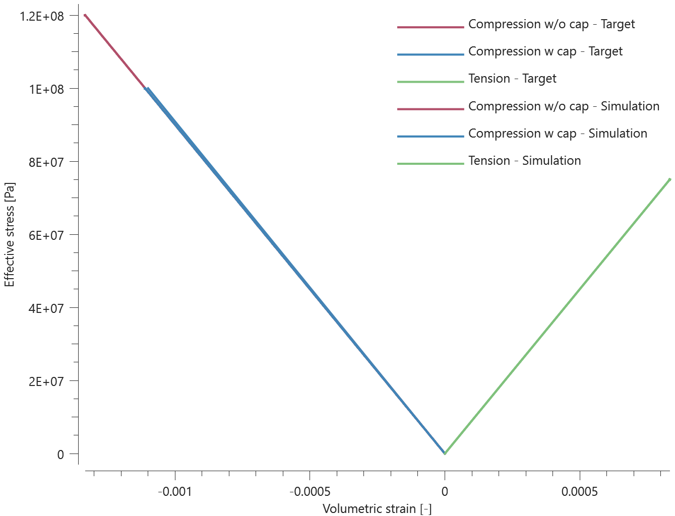
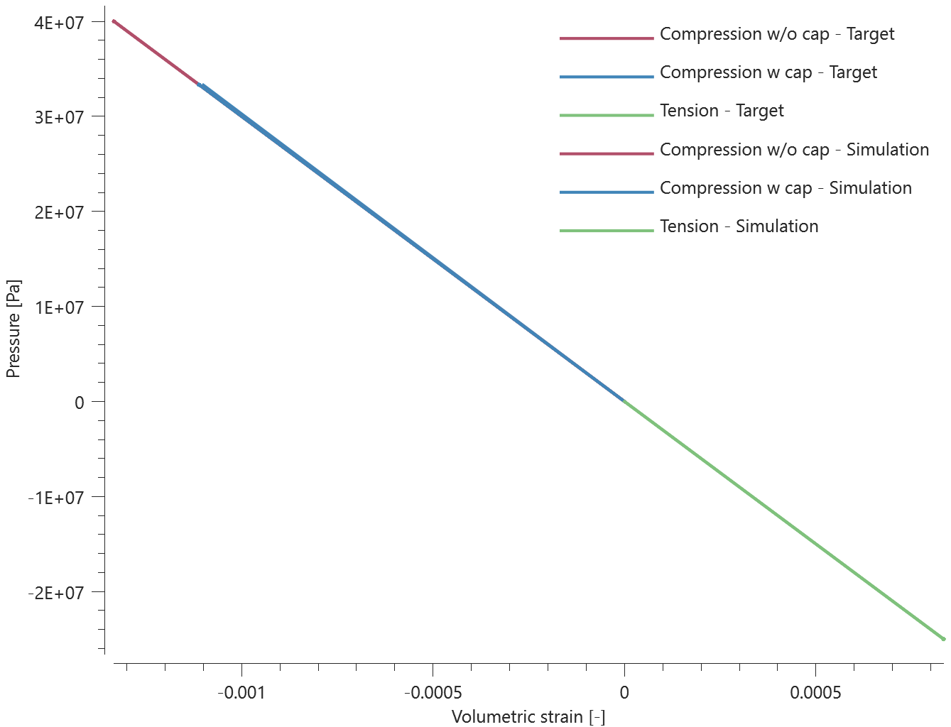
Effective stress vs. volumetric strain and pressure vs. volumetric strain from the SPH test are presented in Figure 3 and 4 together with targets based on the calculations above.
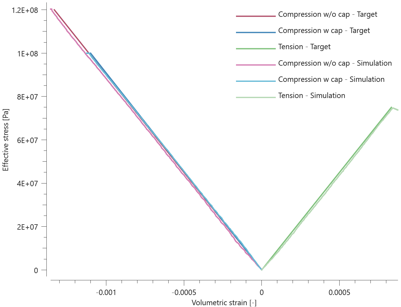
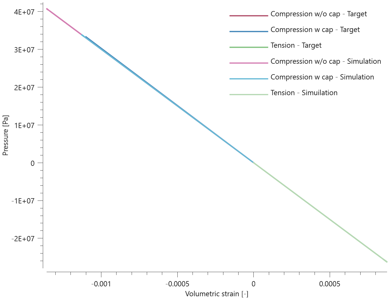
Maximum, minimum and average effective stress, pressure and volumetric strain are checked in the elements. The test was initially only carried out for a CHEX element, hence it is not an optimal test for SPH. This explains the discripancies in the result for SPH. However, to test the functionality of the material model with SPH this is deemed acceptable.
Tests
This benchmark is associated with 2 tests.
*MAT_HJC_CONCRETE
Uniaxial compression followed by unloading
"Optional title"
mid, $\rho$, $G$
$A$, $B$, $n$, $C$, $f_c$, $T$, $\dot\varepsilon_0$, $ef_{min}$
$sf_{max}$, $p_{\mathrm{c}}$, $\mu_{\mathrm{c}}$, $p_{\mathrm{l}}$, $\mu_{\mathrm{l}}$, $D_1$, $D_2$, $K_1$
$K_2$, $K_3$, erode
The command *MAT_HJC_CONCRETE is verified in this test.
A CHEX element is loaded in uniaxial compression followed by unloading.
Maximum and average effective stress, damage and pressure is checked for version control.
Tests
This benchmark is associated with 1 tests.
*MAT_HSS
Abdiabatic shear bands - SPH
"Optional title"
mid, $\rho$, $E$, $\nu$, did, tid
$A$, $B$, $n$, $c$, $c_{dec}$, $s$, $m$
$\dot{\varepsilon}_s$, ${\varepsilon}_s$, $c_s$, ${\eta}_s$, $T^{max}_s$
$c_r$, $\dot{\varepsilon}_r$
The abdiabatic shear properties of *MAT_HSS using SPH particles are verified in this test.
Tested parameters: $\dot{\varepsilon}_s$, ${\varepsilon}_s$, $c_s$ and ${\eta}_s$.
A cube of SPH particles is stretched in the X-direction, twice at different strain rates. In order to activate the adiabatic shear bands a higher strain rate is needed. The first test is therefore done at a too low strain rate, while the second test will active the abdiabatic shear bands. Effective plastic stress vs. effective plastic strain is compared to target curves in Figure 1, without abdiabatic shear bands, and Figure 2, with abdiabatic shear bands.
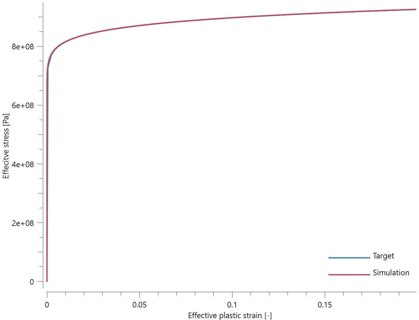
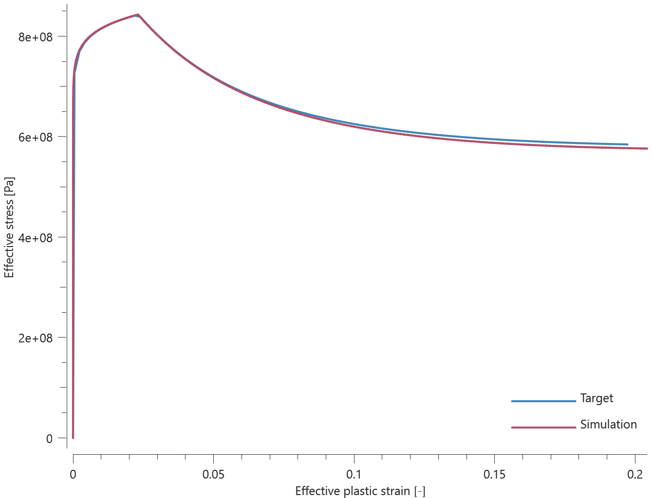
Last values of effective plastic stress and effective plastic strain are checked in both cases.
Tests
This benchmark is associated with 2 tests.
Characteristic element size
"Optional title"
mid, $\rho$, $E$, $\nu$, did, tid
$A$, $B$, $n$, $c$, $c_{dec}$, $s$, $m$
$\dot{\varepsilon}_s$, ${\varepsilon}_s$, $c_s$, ${\eta}_s$, $T^{max}_s$
$c_r$, $\dot{\varepsilon}_r$
The characteristic element size in *MAT_HSS is verified in this test.
Two CHEX elements are stretched in the Z-direction while free in the X- and Y-direction. For one of the elements the combination of strength differential effects, Hosford yield surface exponent and adiabatic softening is activated.
Effective stress vs. effective plastic strain from both elements are presented in Figure 1 together with target curves from a verification script.
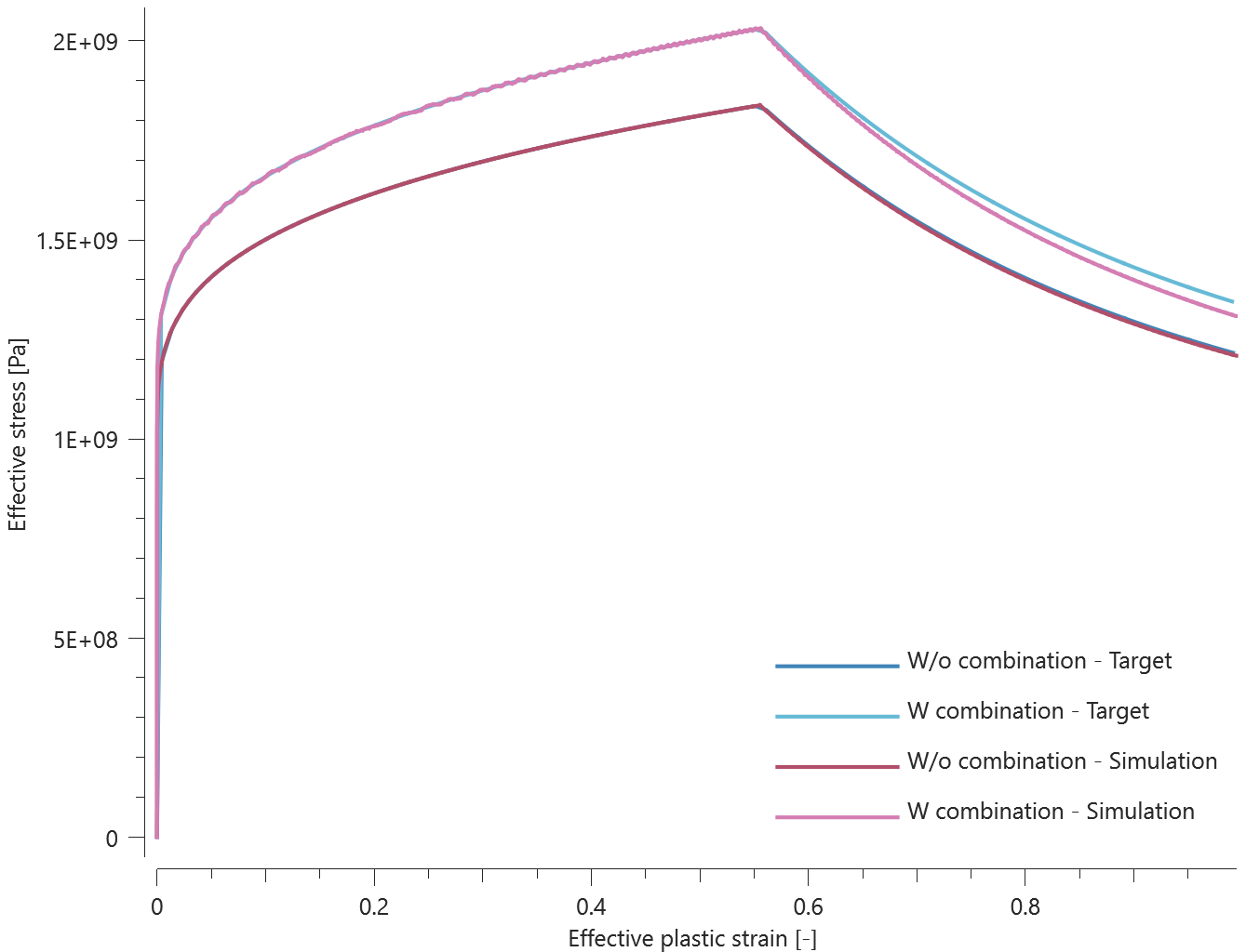
Maximum and average effective stress and effective plastic strain are checked in the elements.
Tests
This benchmark is associated with 1 tests.
Constant parameters yield stress - SPH
"Optional title"
mid, $\rho$, $E$, $\nu$, did, tid
$A$, $B$, $n$, $c$, $c_{dec}$, $s$, $m$
$\dot{\varepsilon}_s$, ${\varepsilon}_s$, $c_s$, ${\eta}_s$, $T^{max}_s$
$c_r$, $\dot{\varepsilon}_r$
The temperature dependent yield stress of *MAT_HSS using SPH particles is verified in this test.
Tested parameters: $\nu$, $A$, $B$, and $n$.
A cube of SPH particles is stretched in the X-direction. The yield stress parameters are defined as functions of temperature. Effective plastic stress vs. effective plastic strain and temperature vs time from a sensor placed centrally in the cube are compared to target curves in Figure 1.
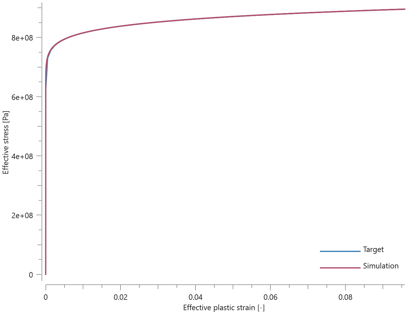
Last value of effective plastic strain and effective plastic stress in the sensor are checked.
Tests
This benchmark is associated with 1 tests.
Dynamic softening
"Optional title"
mid, $\rho$, $E$, $\nu$, did, tid
$A$, $B$, $n$, $c$, $c_{dec}$, $s$, $m$
$\dot{\varepsilon}_s$, ${\varepsilon}_s$, $c_s$, ${\eta}_s$, $T^{max}_s$
$c_r$, $\dot{\varepsilon}_r$
The dynamic softening effect in *MAT_HSS is verified in this test.
Tested parameters: $\dot{\varepsilon}_s$, $\varepsilon_s$, $c_s$, $\eta_s$ and $T^{max}_s$.
Two CHEX elements are loaded in uniaxial tension. The temperature is above the temperature cap in one of the elements, meaning that the dynamic softening should not be activated for this element.
Effective stress vs. effective plastic strain from both elements are presented in Figure 1 together with target curves from a verification script.
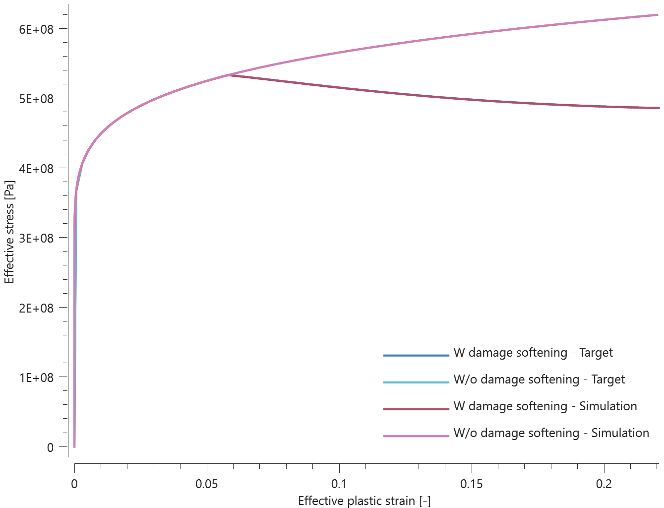
Maximum and average effective stress and effective plastic strain are checked in the elements.
Tests
This benchmark is associated with 1 tests.
JC Damage - SPH
    <div class="manual-structure-box" id="MAT_HSS">
<kbd>
    <span class='nobr'>
    <span>*MAT_HSS</span>
    <br />"Optional title"
    <br />
    <span title="1, 1">mid</span>,
    <span title="1, 2">$\rho$</span>,
    <span title="1, 3">$E$</span>,
    <span title="1, 4">$\nu$</span>,
    <span title="1, 5">did</span>,
    <span title="1, 6">tid</span>
    <br />
    <span title="2, 1">$A$</span>,
    <span title="2, 2">$B$</span>,
    <span title="2, 3">$n$</span>,
    <span title="2, 4">$c$</span>,
    <span title="2, 5">$c_{dec}$</span>,
    <span title="2, 6">$s$</span>,
    <span title="2, 7">$m$</span>
    <br />
    <span title="3, 1">$\dot{\varepsilon}_s$</span>,
    <span title="3, 2">${\varepsilon}_s$</span>,
    <span title="3, 3">$c_s$</span>,
    <span title="3, 4">${\eta}_s$</span>,
    <span title="3, 5">$T^{max}_s$</span>
    <br />
    <span title="4, 1">$c_r$</span>,
    <span title="4, 2">$\dot{\varepsilon}_r$</span></span>
</kbd>
This tests the use of a damage and failure criterion for *MAT_HSS when modelling with SPH particles.
A cube of SPH particles is stretched in the X-direction until failure occurs. Damage vs. effective plastic strain and effective plastic stress vs. effective plastic strain are compared to target curves in Figure 1 and Figure 2.
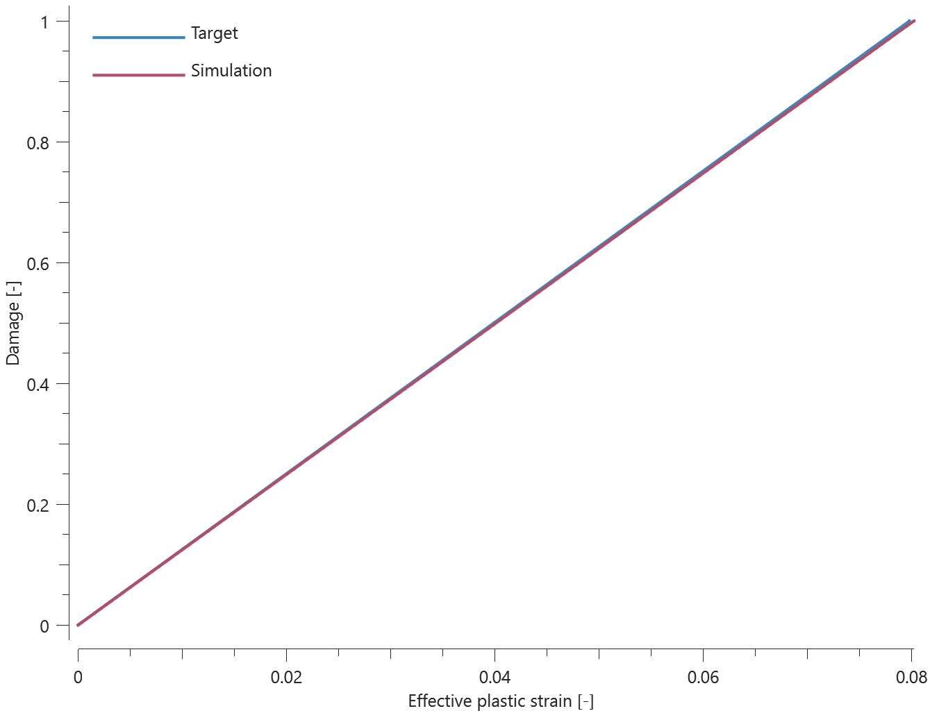
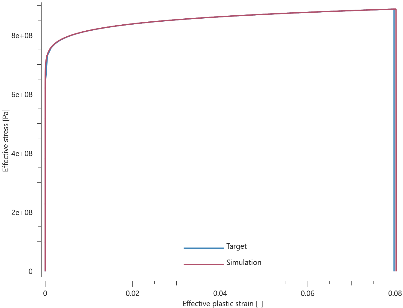
Last values of effective plastic stress, effective plastic strain and damage are checked, as well as maximum and average values for effective plastic stress.
Tests
This benchmark is associated with 1 tests.
Plastic work to heat conversion
"Optional title"
mid, $\rho$, $E$, $\nu$, did, tid
$A$, $B$, $n$, $c$, $c_{dec}$, $s$, $m$
$\dot{\varepsilon}_s$, ${\varepsilon}_s$, $c_s$, ${\eta}_s$, $T^{max}_s$
$c_r$, $\dot{\varepsilon}_r$
The heat conversion from plastic work is tested with this test.
A LHEX element is stretched in X-direction. Temperature vs effective plastic strain is compared in Figure 1 together with target curves from a verification script.
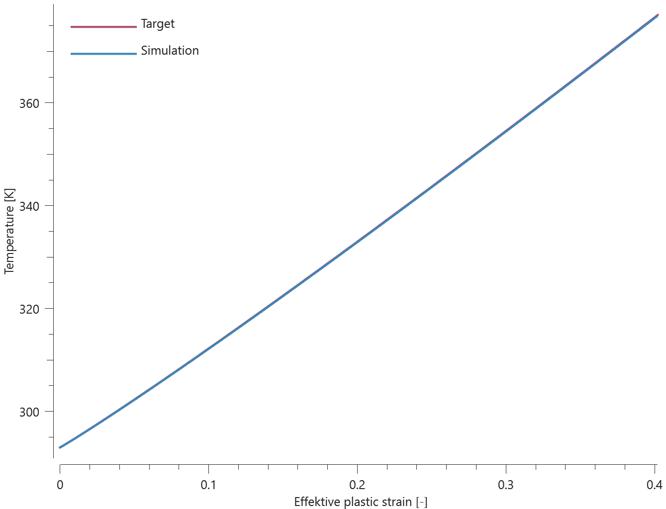
Effective stress vs. effective plastic strain from the element are displayed in Figure 2 together with target curves from a verification script.

Maximum, minimum and average values for temperature, effective plastic strain and effective stress are checked.
Tests
This benchmark is associated with 1 tests.
Strain rate hardening - SPH
"Optional title"
mid, $\rho$, $E$, $\nu$, did, tid
$A$, $B$, $n$, $c$, $c_{dec}$, $s$, $m$
$\dot{\varepsilon}_s$, ${\varepsilon}_s$, $c_s$, ${\eta}_s$, $T^{max}_s$
$c_r$, $\dot{\varepsilon}_r$
The strain rate hardening of *MAT_HSS using SPH particles is verified in this test.
Tested parameters: $c_r$ and $\dot{\varepsilon}_r$.
A cube of SPH particles is stretched in the X-direction. Loading is caused by a prescribed strain rate which with the defined rate parameters influence the yield stress. Effective plastic stress vs. effective plastic strain from a sensor placed centrally in the cube are compared to target curves in Figure 1.
Last value of effective plastic strain and effective plastic stres in the sensor are checked.
Tests
This benchmark is associated with 1 tests.
Strength differential - SPH
"Optional title"
mid, $\rho$, $E$, $\nu$, did, tid
$A$, $B$, $n$, $c$, $c_{dec}$, $s$, $m$
$\dot{\varepsilon}_s$, ${\varepsilon}_s$, $c_s$, ${\eta}_s$, $T^{max}_s$
$c_r$, $\dot{\varepsilon}_r$
The strength differential effect of *MAT_HSS using SPH particles are verified in this test.
Tested parameter: $s$.
A cube of SPH particles is subject for uniaxial tension, as well as uniaxial compression in two seperate tests. The selected strength differential parameter has a significant effect on the yield stress. Effective plastic stress vs. effective plastic strain from a sensor placed centrally in the cube are compared to target curves in Figure 1 and Figure 2.
Last values of effective stress and effective strain are checked in both tests.
Tests
This benchmark is associated with 2 tests.
Strength differential and rate parameters
"Optional title"
mid, $\rho$, $E$, $\nu$, did, tid
$A$, $B$, $n$, $c$, $c_{dec}$, $s$, $m$
$\dot{\varepsilon}_s$, ${\varepsilon}_s$, $c_s$, ${\eta}_s$, $T^{max}_s$
$c_r$, $\dot{\varepsilon}_r$
The strength differential and rate effects of *MAT_HSS are verified in this test.
Tested parameters: $s$, $c_r$ and $\dot{\varepsilon}_r$.
Two CHEX elements are used in this test. One of the elements are loaded in uniaxial tension and the other in uniaxial compression. Loading is caused by a prescribed strain rate which with the defined rate parameters influence the yield stress. The selected strength differential parameter also has a significant effect on the yield stress.
Effective stress vs. effective plastic strain from both elements are presented in Figure 1 together with target curves from a verification script.
Maximum and average effective stress and effective plastic strain are checked for both elements.
Tests
This benchmark is associated with 1 tests.
Temperature dependent elasticity
"Optional title"
mid, $\rho$, $E$, $\nu$, did, tid
$A$, $B$, $n$, $c$, $c_{dec}$, $s$, $m$
$\dot{\varepsilon}_s$, ${\varepsilon}_s$, $c_s$, ${\eta}_s$, $T^{max}_s$
$c_r$, $\dot{\varepsilon}_r$
The temperature dependent elasiticity of *MAT_HSS is verified in this test.
Tested parameters: $E$ and $\nu$ as functions of temperature.
A CHEX element is stretched in the Z-direction while fixed in X- and Y-direction. The elastic parameters are defined as functions of temperature. Stress in X-, Y- and Z-direction vs. time from the elements are compared to target curves in Figure 1.
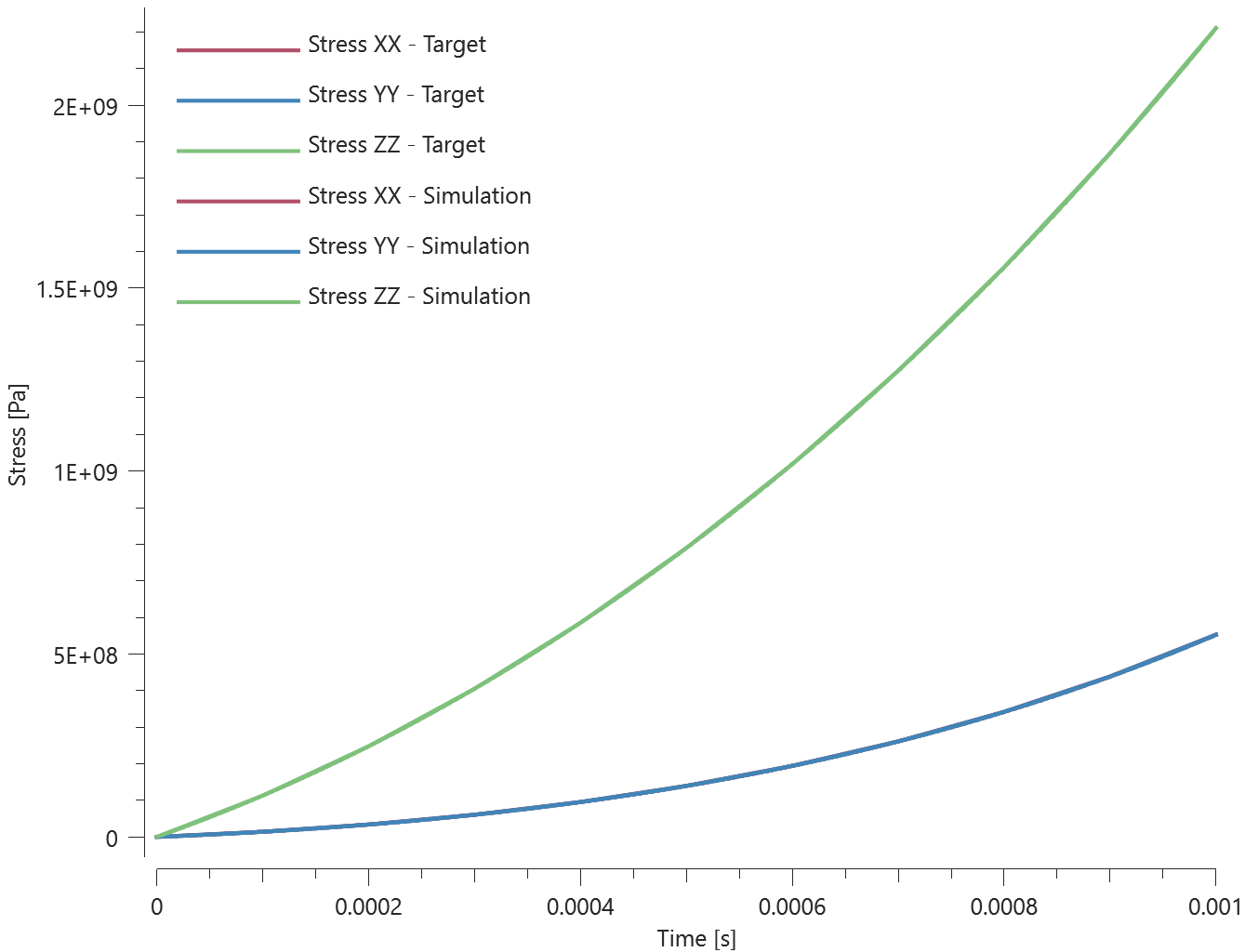
Maximum and average stress in X-, Y- and Z-direction are checked.
Tests
This benchmark is associated with 1 tests.
Temperature dependent elasticity- SPH
"Optional title"
mid, $\rho$, $E$, $\nu$, did, tid
$A$, $B$, $n$, $c$, $c_{dec}$, $s$, $m$
$\dot{\varepsilon}_s$, ${\varepsilon}_s$, $c_s$, ${\eta}_s$, $T^{max}_s$
$c_r$, $\dot{\varepsilon}_r$
The temperature dependent elasiticity of *MAT_HSS using SPH particles is verified in this test. The test is done twice, once for T = 293K and once for T = 493K.
Tested parameters: $E$ and $\nu$ as functions of temperature.
A cube of SPH particles is stretched in the Z-direction while fixed in X- and Y-direction. The elastic parameters are defined as functions of temperature. Effective stress vs. volumetric strain from the middle of the cube are compared to target curves in Figure 1.
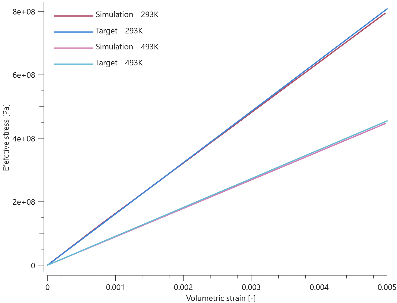
Last values of effective stress and volumetric strain are checked.
Tests
This benchmark is associated with 2 tests.
Temperature dependent yield stress - SPH
"Optional title"
mid, $\rho$, $E$, $\nu$, did, tid
$A$, $B$, $n$, $c$, $c_{dec}$, $s$, $m$
$\dot{\varepsilon}_s$, ${\varepsilon}_s$, $c_s$, ${\eta}_s$, $T^{max}_s$
$c_r$, $\dot{\varepsilon}_r$
The temperature dependent yield stress of *MAT_HSS using SPH particles is verified in this test.
Tested parameters: $A$, $B$ and $n$ as functions of temperature.
A cube of SPH particles is stretched in the X-direction. The yield stress parameters are defined as functions of temperature. Effective plastic stress vs. effective plastic strain and temperature vs effective plastic strain from a sensor placed centrally in the cube are compared to target curves in Figure 1. Temperature vs. effective plastic strain are compared against a target in Figure 2.
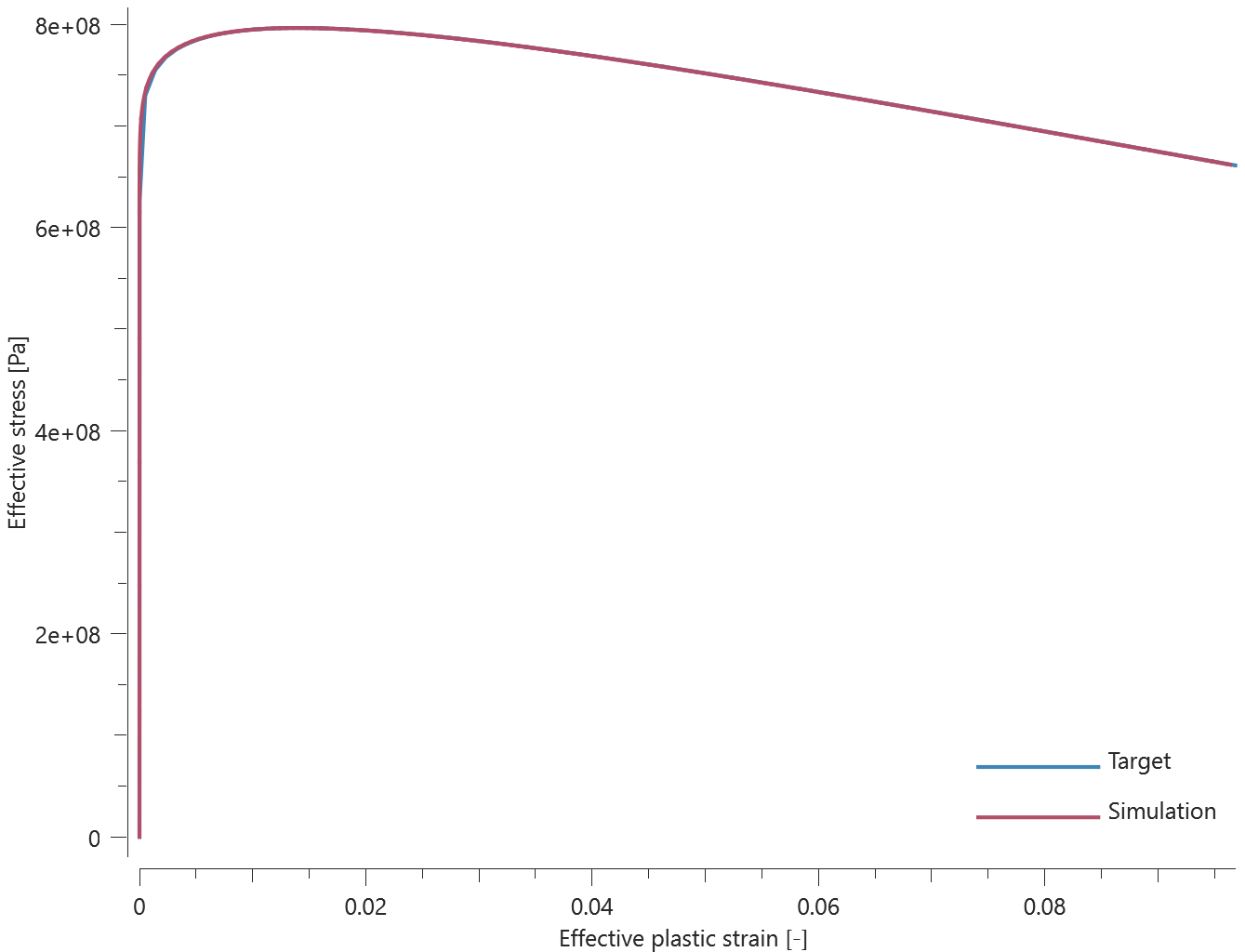
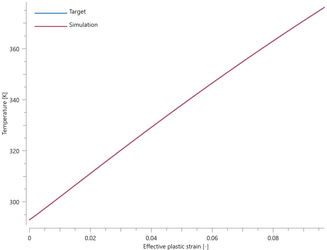
Last value of effective plastic strain, effective plastic stress and temperature in the sensor are checked.
Tests
This benchmark is associated with 1 tests.
Viscosity
"Optional title"
mid, $\rho$, $E$, $\nu$, did, tid
$A$, $B$, $n$, $c$, $c_{dec}$, $s$, $m$
$\dot{\varepsilon}_s$, ${\varepsilon}_s$, $c_s$, ${\eta}_s$, $T^{max}_s$
$c_r$, $\dot{\varepsilon}_r$
The viscosity in *MAT_HSS is verifed in this test.
Tested parameters: $c$ and $c_{dec}$.
Three CHEX elements are used in this model, one for each input option of the viscous parameter (constant, curve and function). The viscocity is defined as independent of strain rate for all cases, and different values are used for each element.
Effective stress vs. effective plastic strain from the elements are displayed in Figure 1 together with target curves from a verification script.
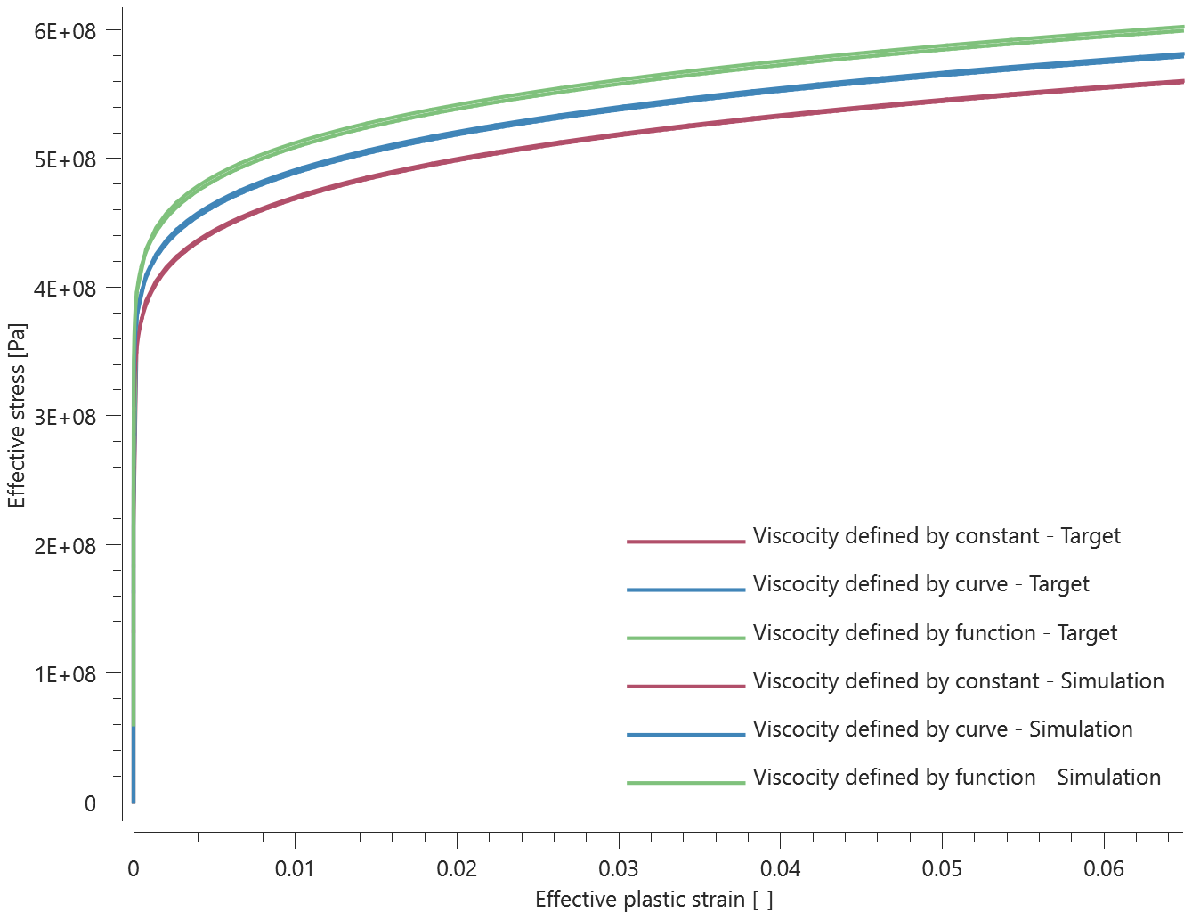
Maximum and average effective stress and effective plastic strain are checked in the elements.
Tests
This benchmark is associated with 1 tests.
Yield stress
"Optional title"
mid, $\rho$, $E$, $\nu$, did, tid
$A$, $B$, $n$, $c$, $c_{dec}$, $s$, $m$
$\dot{\varepsilon}_s$, ${\varepsilon}_s$, $c_s$, ${\eta}_s$, $T^{max}_s$
$c_r$, $\dot{\varepsilon}_r$
The yield strength and strain hardening parameters of *MAT_HSS is verified in this test.
Tested parameters: $A$, $B$ and $n$ entered as constants and as functions of temperature.
Two CHEX elements are used in this model. The yield stress parameters are entered as constants in one of the elements and as functions of temperature in the other. The elements are stretched in the X-direction while fixed in the Y- and Z-direction.
Effective stress vs. effective plastic strain from the elements are presented in Figure 1 together with target curves from a verification script.
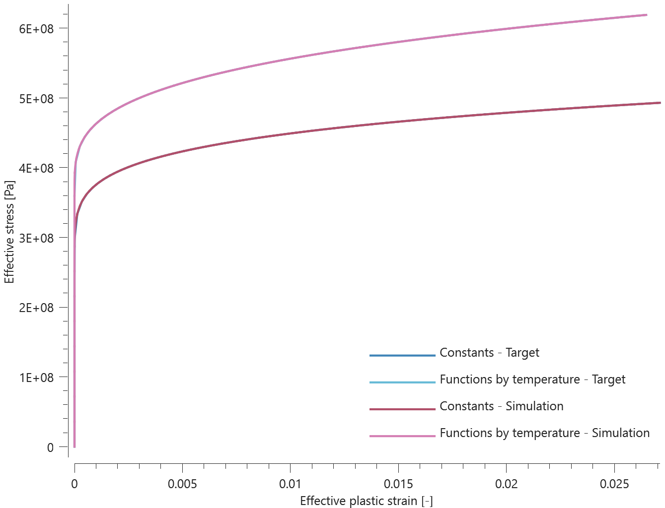
Maximum and average effective stress and effective plastic strain are checked in the elements.
Tests
This benchmark is associated with 1 tests.
Yield surface
"Optional title"
mid, $\rho$, $E$, $\nu$, did, tid
$A$, $B$, $n$, $c$, $c_{dec}$, $s$, $m$
$\dot{\varepsilon}_s$, ${\varepsilon}_s$, $c_s$, ${\eta}_s$, $T^{max}_s$
$c_r$, $\dot{\varepsilon}_r$
The yield surface of *MAT_HSS is verified in this test.
Tested parameter: $m$.
A CHEX element is subjected to a number of different uniaxial and biaxial loading cases. Two different values of Hosford yield surface exponent are investigated: 0 (von Mises) and 11.
The principal stresses once the yield surface is reached are extracted from the simulations and plotted in Figure 1 together with the yield surfaces used in the simulations.
The principal stresses at termination are checked.
Tests
This benchmark is associated with 24 tests.
*MAT_JC
Quasi-static yield stress
"Optional title"
mid, $\rho$, $E$, $\nu$, did, tid, eosid
$A$, $B$, $n$, $C$, $m$, $T_0$, $T_m$, $\dot{\varepsilon}_0$
$C_p$, $k$, $d$, $e$
The quasi-static yield strength and strain hardening in *MAT_JC are verified in this test.
Tested parameters: $A$, $B$ and $n$.
A CHEX element, as well as a SPH cubic box, is loaded in uniaxial tension. Effective stress vs. effective plastic strain from the element and the SPH cube is presented in Figure 1 together with a target curve.
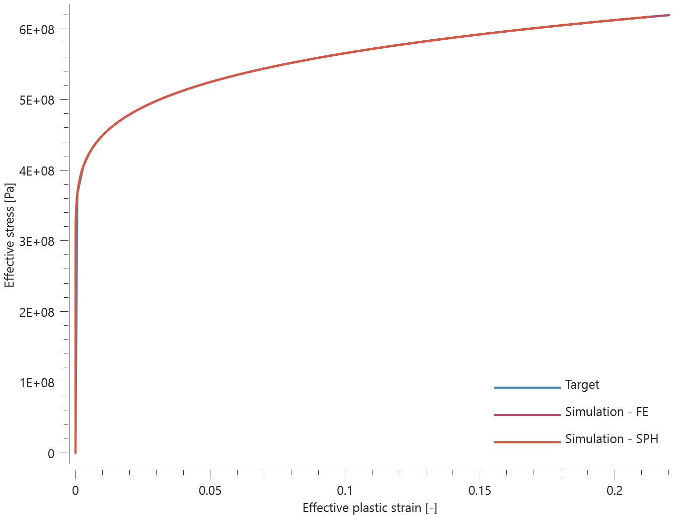
Maximum and average effective stress and effective plastic strain are checked.
Tests
This benchmark is associated with 2 tests.
Strain rate effect
"Optional title"
mid, $\rho$, $E$, $\nu$, did, tid, eosid
$A$, $B$, $n$, $C$, $m$, $T_0$, $T_m$, $\dot{\varepsilon}_0$
$C_p$, $k$, $d$, $e$
The strain rate effect in *MAT_JC is verified in this test.
Tested parameters: $C$ and $\dot{\varepsilon}_0$.
A CHEX element is loaded in uniaxial tension. Effective stress vs. effective plastic strain from the element is presented in Figure 1.
The test is also done with a SPH cubic geometry, and that result can be found in Figure 2 together with a target curve from a verification script.
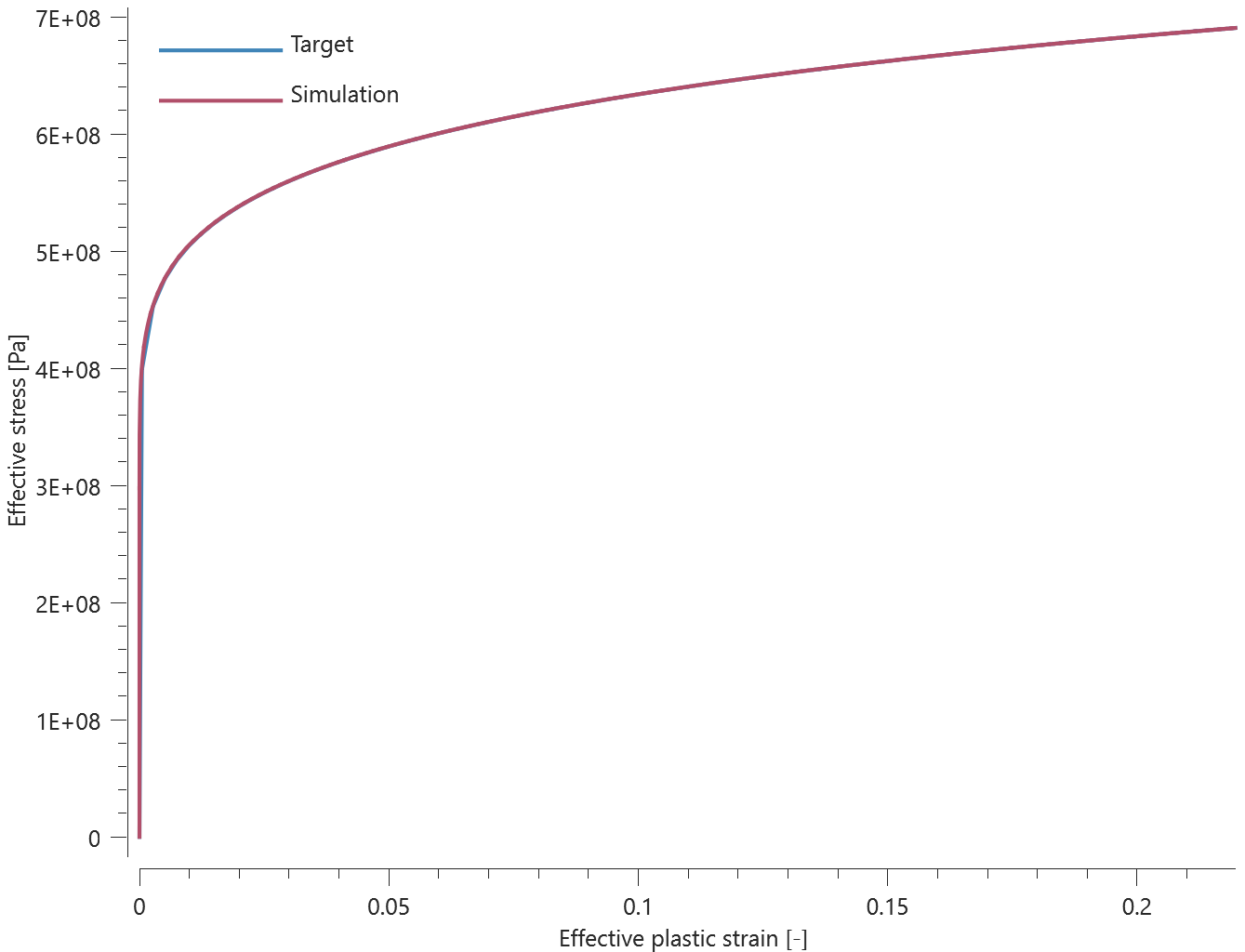
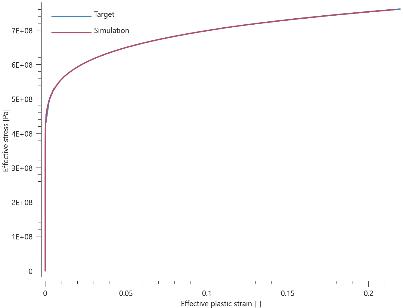
To reduce the computational time the SPH simulation is done with a higher velocity than the CHEX. Hence the difference in target curves.
Maximum and average effective stress and effective plastic strain are checked.
Tests
This benchmark is associated with 2 tests.
Thermal softening effect
"Optional title"
mid, $\rho$, $E$, $\nu$, did, tid, eosid
$A$, $B$, $n$, $C$, $m$, $T_0$, $T_m$, $\dot{\varepsilon}_0$
$C_p$, $k$, $d$, $e$
The thermal softening effect in *MAT_JC is verified in this test.
Tested parameters: $m$, $T_0$, $T_m$, $C_p$, $k$, $d$ and $e$.
A CHEX element is loaded in uniaxial tension. Effective stress vs. effective plastic strain and temperature vs. effective plastic strain from the element is presented in Figure 1 and 2 together with a target curves from a verfication script.
The test is also done using surface SPH.
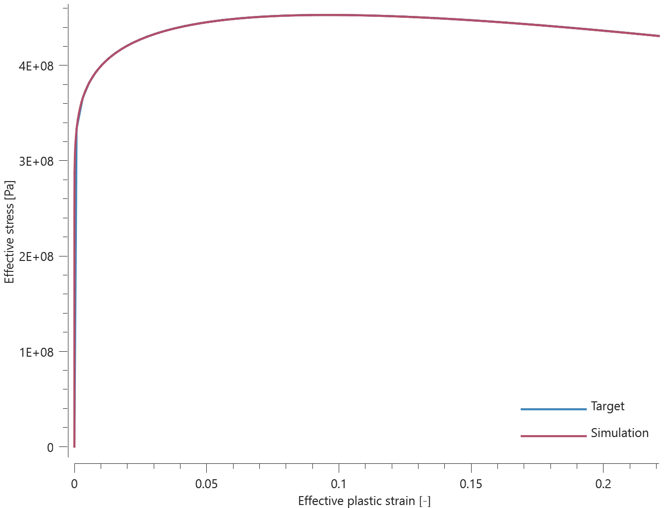
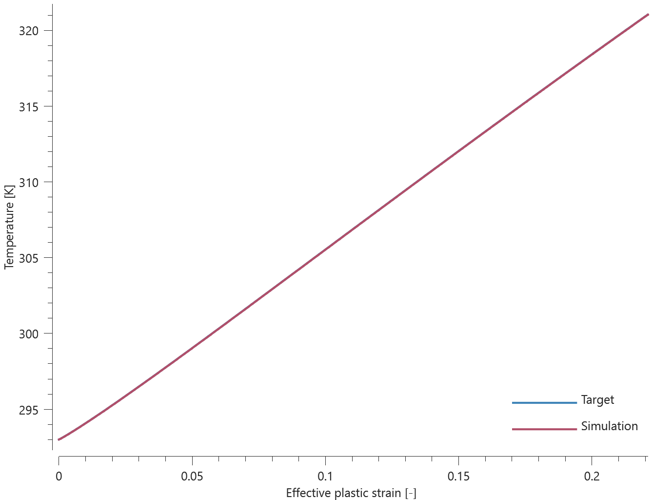
Maximum and average effective stress, temperature and effective plastic strain are checked.
Tests
This benchmark is associated with 2 tests.
*MAT_JC_FIELD
Damage and failure criterion
"Optional title"
mid, $\rho$, $E$, $\nu$
$A$, $B$, $n$, $C$, $m$, $T_0$, $T_m$, $\dot{\varepsilon}_0$
$C_p$, $k$, $W_{c0}$, $c_1$, $c_2$, erode
The damage and failure criterion in *MAT_JC_FIELD are verified in this test.
Tested parameters: $W_{c0}$, $c_1$ and $c_2$.
Two CHEX elements are used in this model. The elements are aligned along the X-axis, with one element located at X > 0 and the other one at X < 0.
A function is defined:
$$ f(X) = 1.0 + 0.1 \cdot sign(X) $$
All parameters used as input to *MAT_JC_FIELD are multiplied with the function, meaning that the input for the element located in X > 0 is a factor 1.1 times the defined parameters, and the input for the element in X < 0 is a factor 0.9 times the defined parameters.
Effective stress vs. effective plastic strain and damage vs. effective plastic strain are presented in Figure 1 and 2 together with target curves from a verification script.
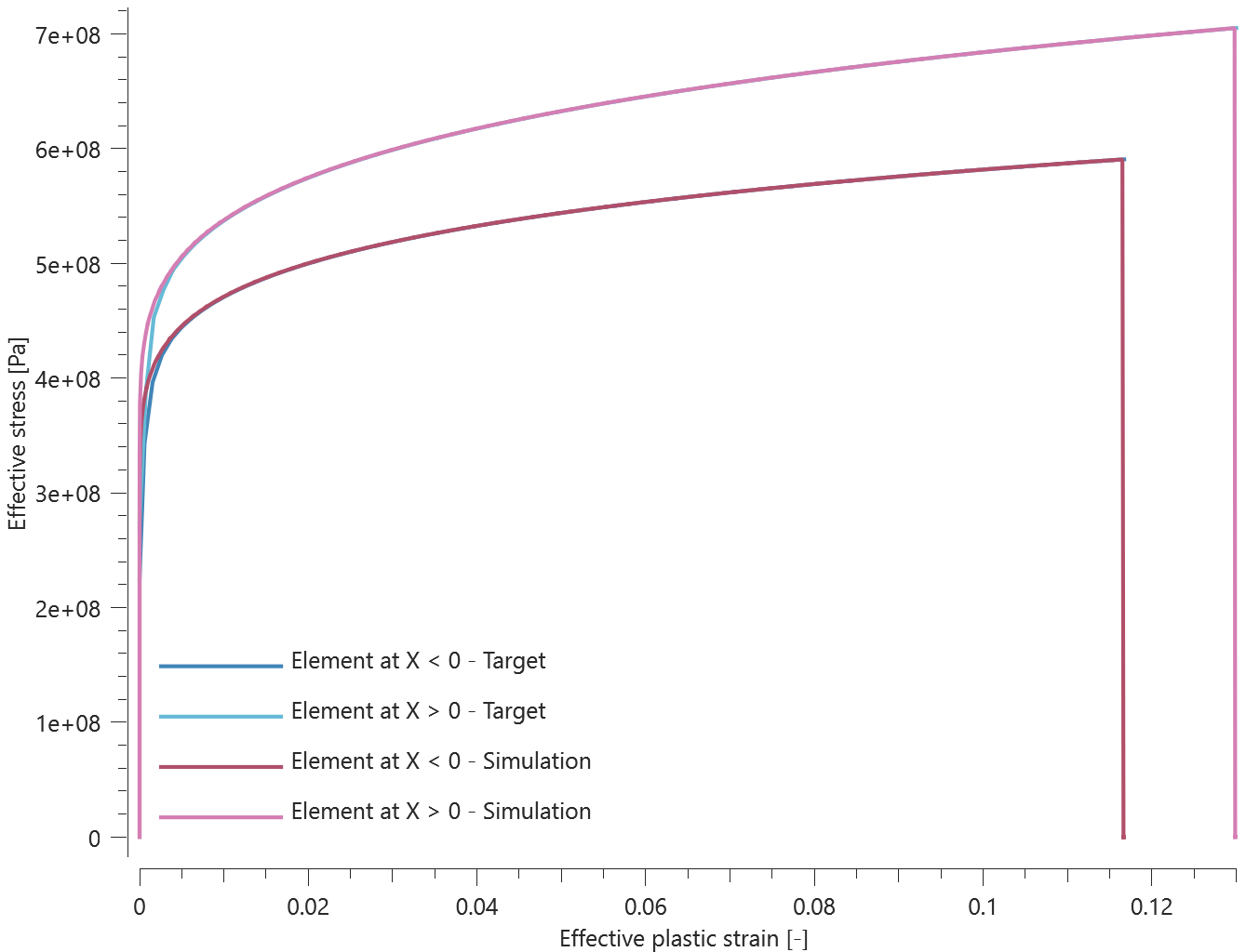
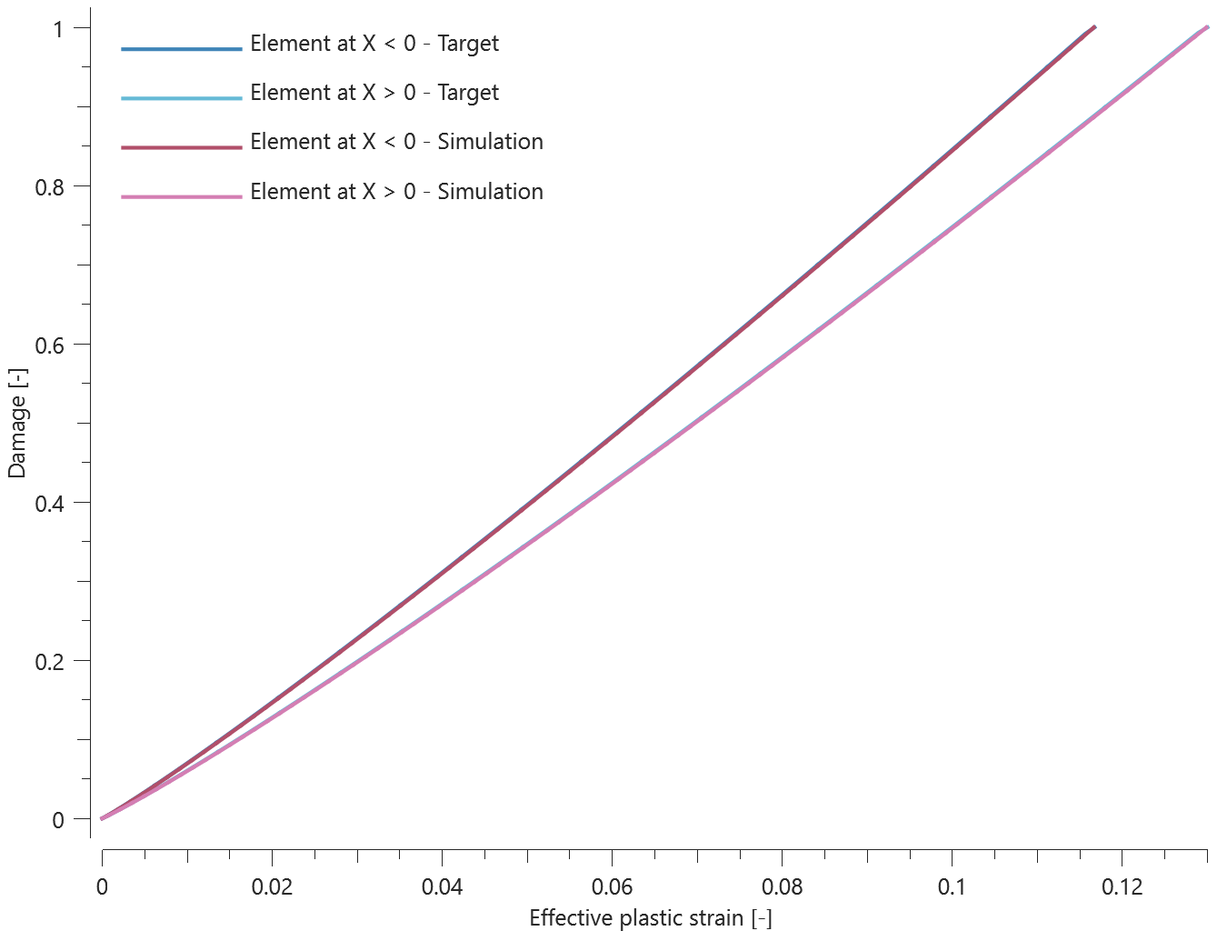
Maximum and average effective stress, effective plastic strain and damage are checked in the elements.
Tests
This benchmark is associated with 1 tests.
Quasi-static yield stress
"Optional title"
mid, $\rho$, $E$, $\nu$
$A$, $B$, $n$, $C$, $m$, $T_0$, $T_m$, $\dot{\varepsilon}_0$
$C_p$, $k$, $W_{c0}$, $c_1$, $c_2$, erode
The yield limit and strain hardening in *MAT_JC_FIELD are verified in this test.
Tested parameters: $A$, $B$ and $n$ (entered as functions).
Two CHEX elements are used in this model. The elements are aligned along the X-axis, with one element located at X > 0 and the other one at X < 0.
A function is defined:
$$ f(X) = 1.0 + 0.1 \cdot sign(X)$$
All parameters used as input to *MAT_JC_FIELD are multiplied with the function, meaning that the input for the element located in X > 0 is a factor 1.1 times the defined parameters, and the input for the element in X < 0 is a factor 0.9 times the defined parameters.
Effective stress vs. effective plastic strain from the elements are presented in Figure 1 together with a target curve from a verification script.
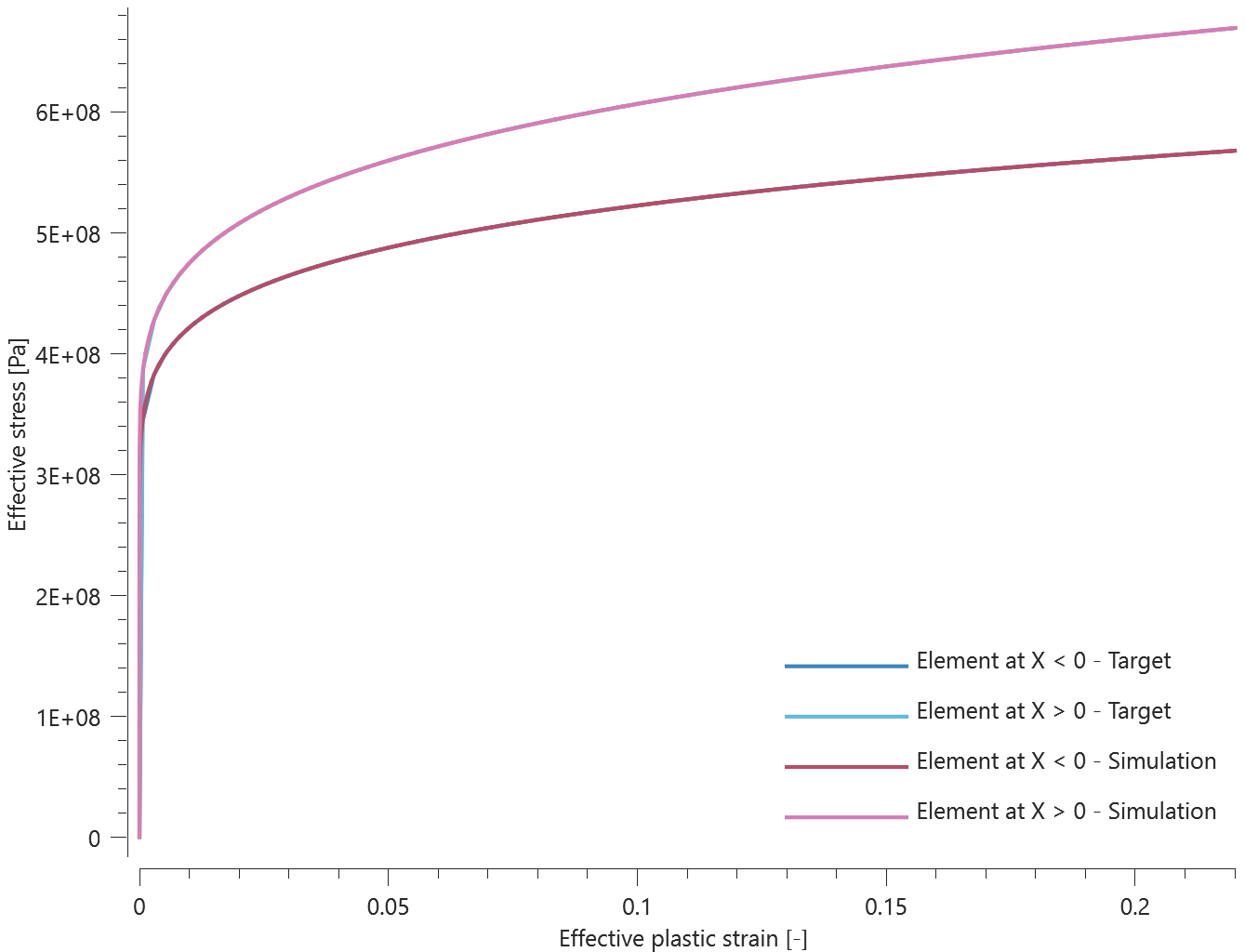
Maximum and average effective stress and effective plastic strain are checked in the elements.
Tests
This benchmark is associated with 1 tests.
Strain rate effect
"Optional title"
mid, $\rho$, $E$, $\nu$
$A$, $B$, $n$, $C$, $m$, $T_0$, $T_m$, $\dot{\varepsilon}_0$
$C_p$, $k$, $W_{c0}$, $c_1$, $c_2$, erode
The strain rate effect in *MAT_JC_FIELD is verified in this test.
Tested parameters: $C$ and $\dot{\varepsilon}_0$.
Two CHEX elements are used in this model. The elements are aligned along the X-axis, with one element located at X > 0 and the other one at X < 0.
A function is defined:
$$ f(X) = 1.0 + 0.1 \cdot sign(X) $$
All parameters used as input to *MAT_JC_FIELD are multiplied with the function, meaning that the input for the element located in X > 0 is a factor 1.1 times the defined parameters, and the input for the element in X < 0 is a factor 0.9 times the defined parameters.
Effective stress vs. effective plastic strain from the elements are presented in Figure 1 together with a target curve from a verification script.
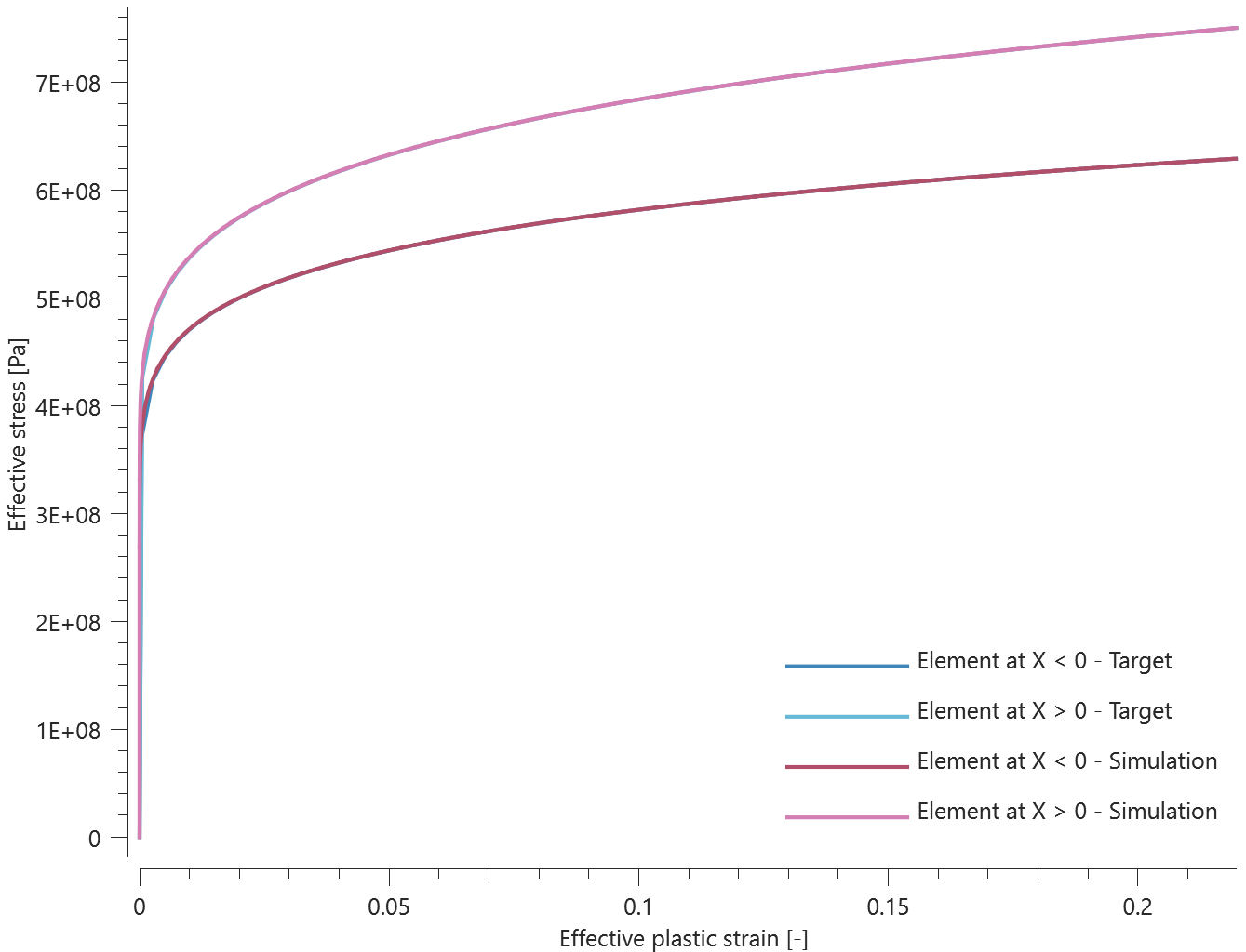
Maximum and average effective stress and effective plastic strain are checked.
Tests
This benchmark is associated with 1 tests.
Thermal softening effect
"Optional title"
mid, $\rho$, $E$, $\nu$
$A$, $B$, $n$, $C$, $m$, $T_0$, $T_m$, $\dot{\varepsilon}_0$
$C_p$, $k$, $W_{c0}$, $c_1$, $c_2$, erode
The thermal softening effect in *MAT_JC_FIELD is verified in this test.
Tested parameters: $m$, $T_0$, $T_m$, $C_p$ and $k$.
Two CHEX elements are used in this model. The elements are aligned along the X-axis, with one element located at X > 0 and the other one at X < 0.
A function is defined:
$$ f(X) = 1.0 + 0.1 \cdot sign(X) $$
All parameters used as input to *MAT_JC_FIELD are multiplied with the function, meaning that the input for the element located in X > 0 is a factor 1.1 times the defined parameters, and the input for the element in X < 0 is a factor 0.9 times the defined parameters.
Effective stress vs. effective plastic strain and temperature vs. effective plastic strain is plotted in Figure 1 and 2 together with target curves from a verification script.
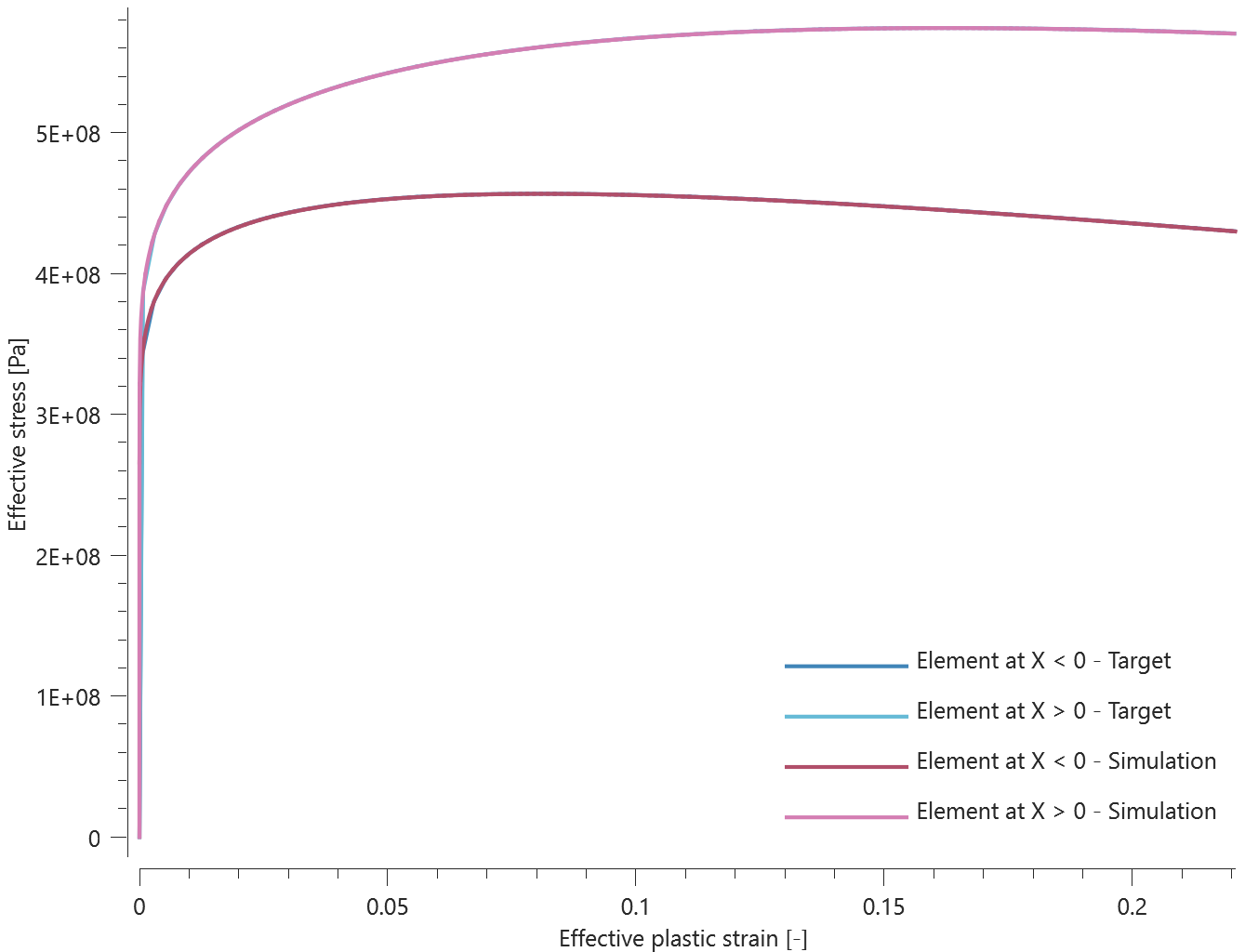
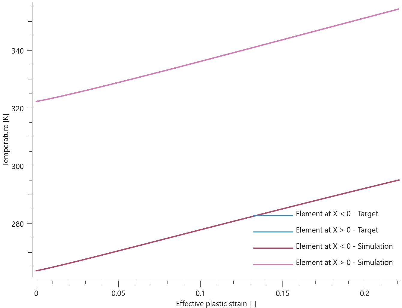
Maximum and average effective stress, effective plastic strain and temperature are checked.
Tests
This benchmark is associated with 1 tests.
*MAT_JH_CERAMIC
Verification
"Optional title"
mid, $\rho$, $G$
$A$, $B$, $C$, $m$, $n$, $\dot{\varepsilon}_0$, $T$
$HEL$, $P_{HEL}$, $\beta$, $D_1$, $D_2$, $K_1$, $K_2$, $K_3$
erode
The three examples presented in the original publication [1] are run to ensure that the material model produces correct results. Effective stress vs. pressure from the simulations are plotted together with data from the original publication in Figure 1-3. A plot digitizer has been used to obtain the data from the original publication.
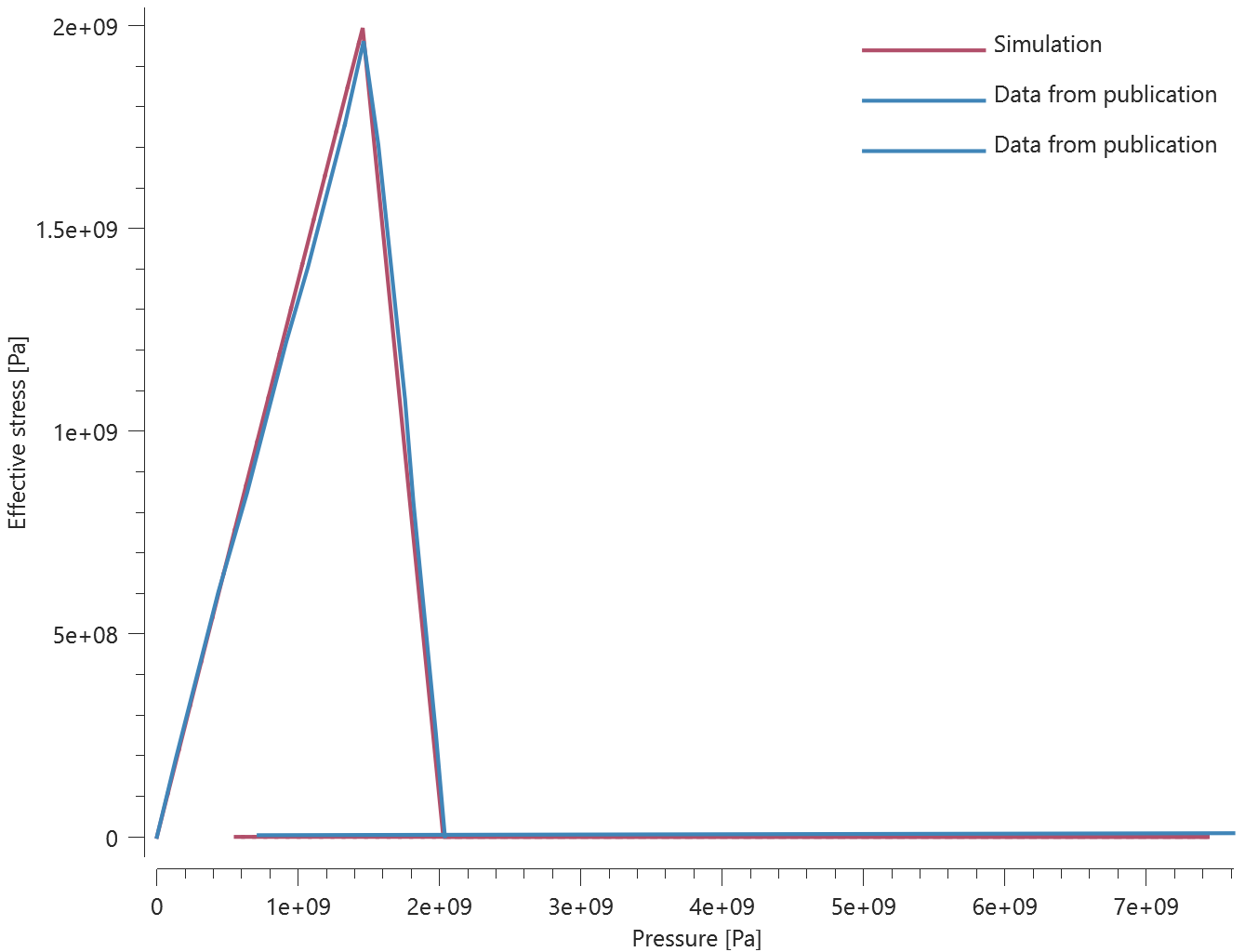
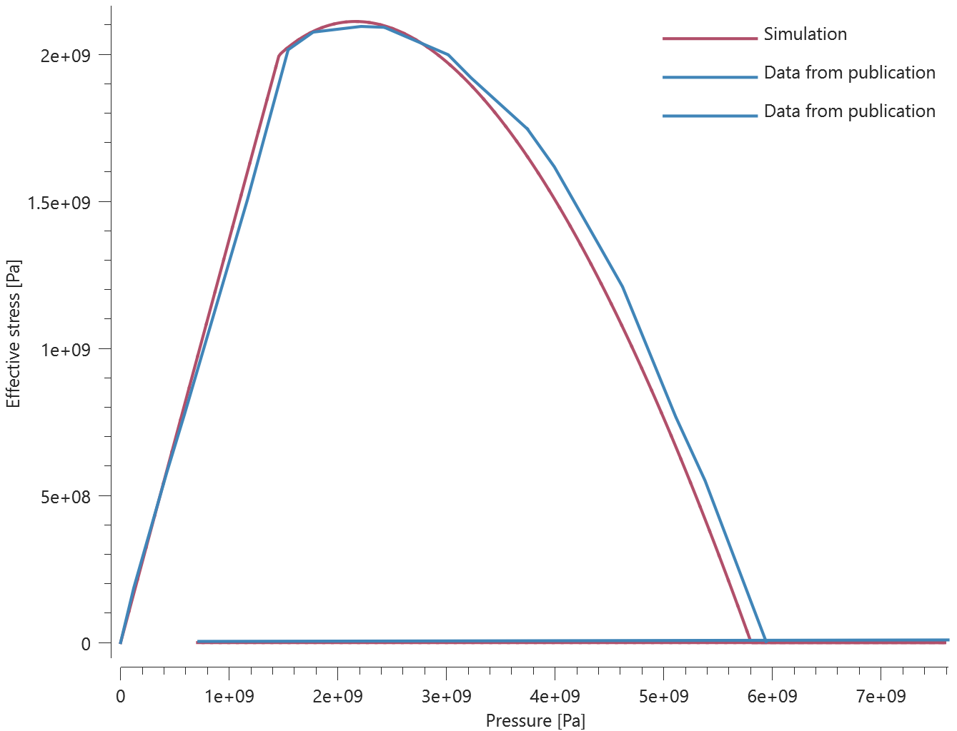
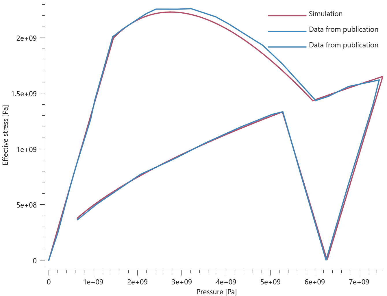
Maximum and average values for effective stress and pressure are checked in each case.
Reference
[1] – G. R. Johnson and T. J. Holmquist – An improved computational constitutive model för brittle materials, American Institute of Physics, 1994.
Tests
This benchmark is associated with 3 tests.
*MAT_METAL
Damage softening
"Optional title"
mid, $\rho$, $E$, $\nu$, did, tid, eosid
cid, $\xi$, tresca, $c$, $\dot\varepsilon_0$, $m$, $T_0$, $T_m$
$s_0$, $s_1$, $\varepsilon_d$, $\mu$
Damage softening in *MAT_METAL is verified in this test.
Tested parameters: $s_0$ and $s_1$.
A CHEX element is loaded in uniaxial tension. Damage is modeled with the command *PROP_DAMAGE_CL. Once the damage reaches the threshold value, $s_0$, damage softening is initiated.
Effective stress vs. effective plastic strain and damage vs. effective plastic strain from the element are displayed in Figure 1 and 2 together with target curves from a verification script.
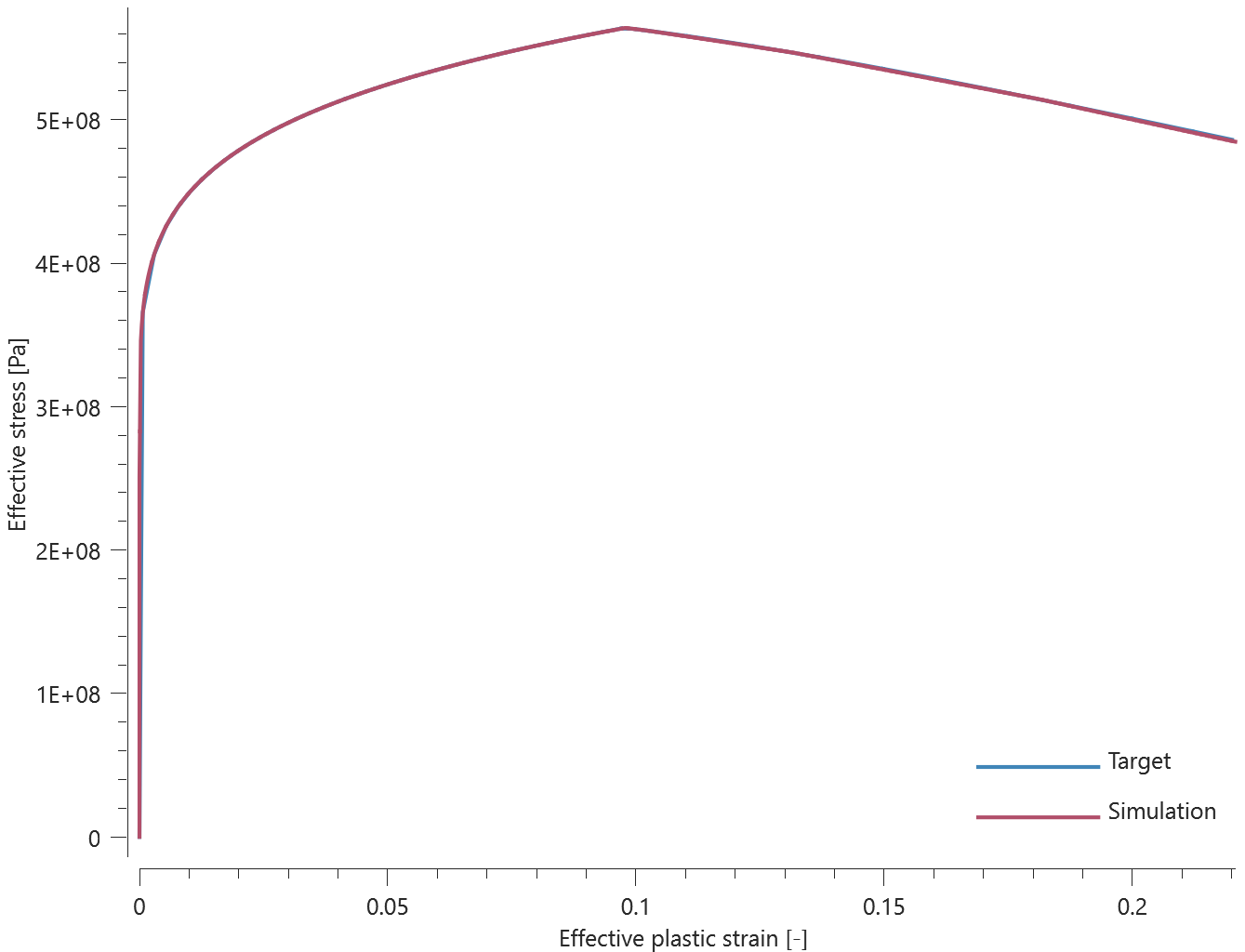
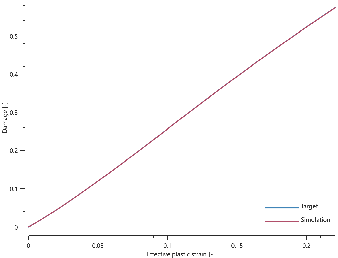
Maximum and average effective stress, effective plastic strain and damage are checked.
Tests
This benchmark is associated with 1 tests.
Decouple rate hardening
"Optional title"
mid, $\rho$, $E$, $\nu$, did, tid, eosid
cid, $\xi$, tresca, $c$, $\dot\varepsilon_0$, $m$, $T_0$, $T_m$
$s_0$, $s_1$, $\varepsilon_d$, $\mu$
The uncoupled strain rate effect in *MAT_METAL is verified in this test.
Tested parameters: $\mu$, $c$ and $\dot{\varepsilon}_0$.
A CHEX element is loaded in uniaxial tension. The static yield strength is defined as zero, $f\left(\varepsilon_{eff}^{p}\right) = 0$. Effective stress vs. effective plastic strain from the element is presented in Figure 1 together with a target curve from a verification script.
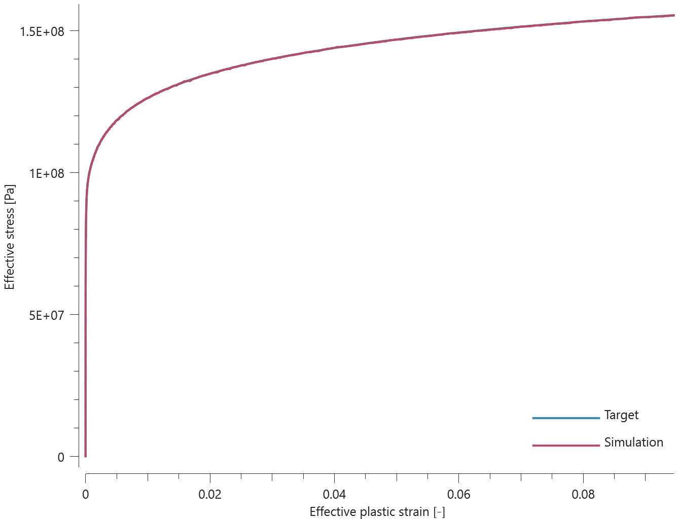
Maximum and average effective stress and effective plastic strain are checked.
Tests
This benchmark is associated with 1 tests.
Isotropic and kinematic hardening
"Optional title"
mid, $\rho$, $E$, $\nu$, did, tid, eosid
cid, $\xi$, tresca, $c$, $\dot\varepsilon_0$, $m$, $T_0$, $T_m$
$s_0$, $s_1$, $\varepsilon_d$, $\mu$
The isotropic and kinematic hardening in *MAT_METAL are verified in this test.
Tested parameters: $E$, $cid$ and $\xi$.
Two CHEX elements are subjected to a cyclic uniaxial load. Isotropic hardening is used in one of the elements and kinematic hardening in the other. Stress in the X-direction vs. time from the elements are presented in Figure 1 and 2 together with target curves from a verification script.
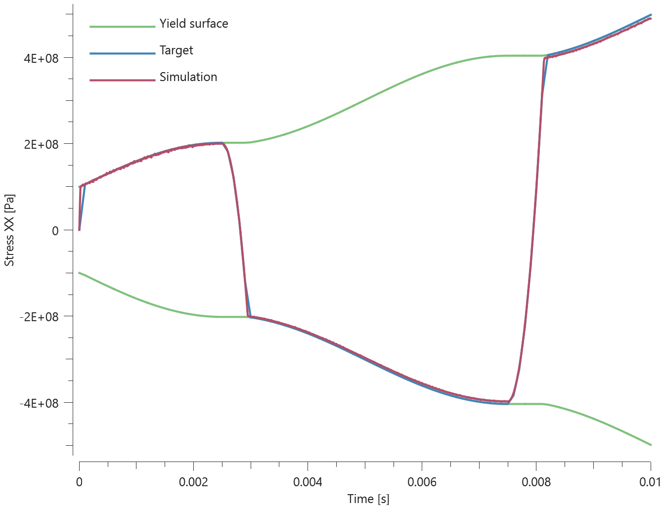
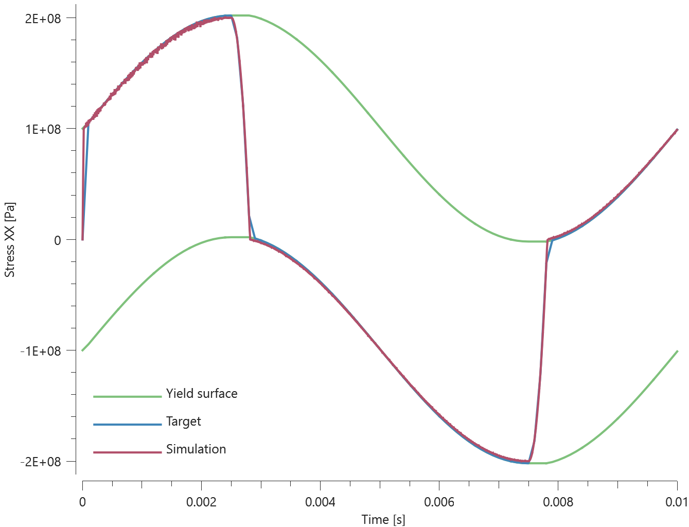
Maximum, minimum and average stress in the loading direction are checked in the elements.
Tests
This benchmark is associated with 1 tests.
Quasi-static yield stress
"Optional title"
mid, $\rho$, $E$, $\nu$, did, tid, eosid
cid, $\xi$, tresca, $c$, $\dot\varepsilon_0$, $m$, $T_0$, $T_m$
$s_0$, $s_1$, $\varepsilon_d$, $\mu$
The yield strength and strain hardening in *MAT_METAL are verified in this test.
Tested parameter: cid (function describing effective stress vs. effective plastic strain).
A CHEX element is loaded in uniaxial tension. Effective stress vs. effective plastic strain from the element is presented in Figure 1 together with a target curve from a verification script.
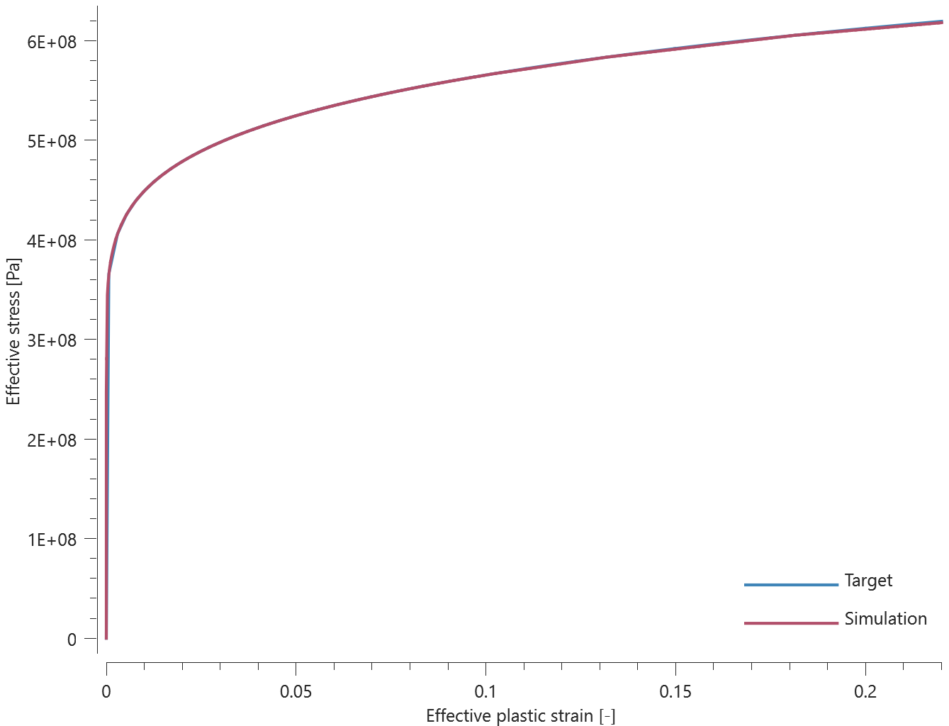
Maximum and average effective stress and effective plastic strain are checked.
Tests
This benchmark is associated with 1 tests.
Strain rate effect
"Optional title"
mid, $\rho$, $E$, $\nu$, did, tid, eosid
cid, $\xi$, tresca, $c$, $\dot\varepsilon_0$, $m$, $T_0$, $T_m$
$s_0$, $s_1$, $\varepsilon_d$, $\mu$
The strain rate effect in *MAT_METAL is verified in this test.
Tested parameters: $c$ and $\dot{\varepsilon}_0$.
A CHEX element is loaded in uniaxial tension. Effective stress vs. effective plastic strain from the element is presented in Figure 1 together with a target curve from a verification script.
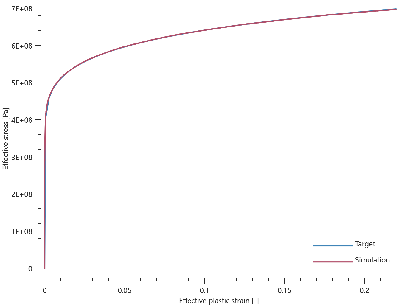
Maximum and average effective stress and effective plastic strain are checked.
Tests
This benchmark is associated with 1 tests.
Thermal softening effect
"Optional title"
mid, $\rho$, $E$, $\nu$, did, tid, eosid
cid, $\xi$, tresca, $c$, $\dot\varepsilon_0$, $m$, $T_0$, $T_m$
$s_0$, $s_1$, $\varepsilon_d$, $\mu$
The thermal softening in *MAT_METAL is verified in this test.
Tested parameters: $m$, $T_0$ and $T_m$.
A CHEX element is loaded in uniaxial tension. Effective stress vs. effective plastic strain and temperature vs. effective plastic strain is presented in Figure 1 and 2 together with target curves from a verification script.
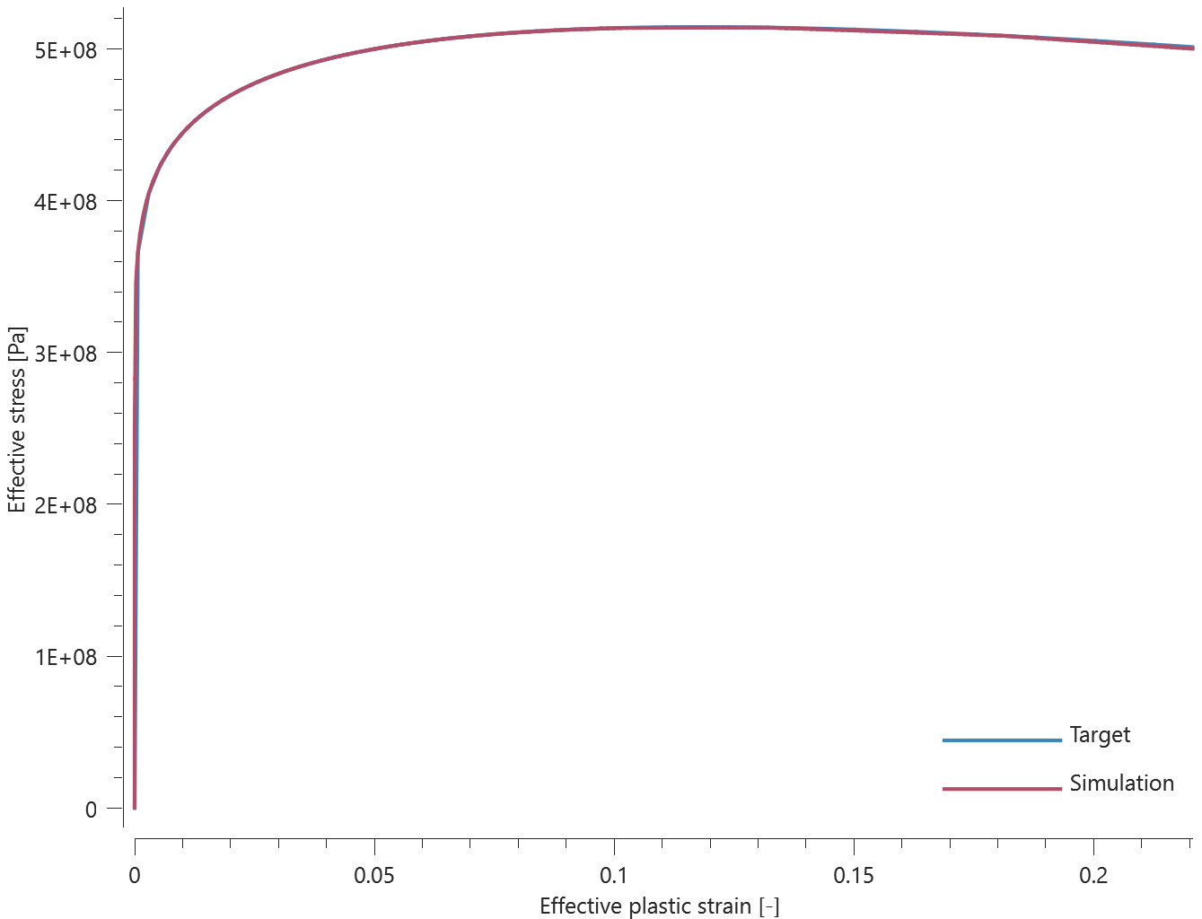
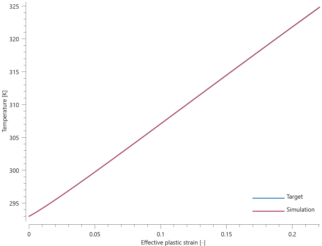
Maximum and average effective stress, effective plastic strain and temperature are checked.
Tests
This benchmark is associated with 1 tests.
Yield surface
"Optional title"
mid, $\rho$, $E$, $\nu$, did, tid, eosid
cid, $\xi$, tresca, $c$, $\dot\varepsilon_0$, $m$, $T_0$, $T_m$
$s_0$, $s_1$, $\varepsilon_d$, $\mu$
The yield surface of *MAT_METAL is verified in this test.
Tested parameter: $tresca$.
A CHEX element is subjected to a number of different uniaxial and biaxial loading cases. Both von Mises (tresca = 0.0) and Tresca's (tresca = 1.0) yield surfaces are investigated.
The principal stresses once the yield surface is reached are extracted from the simulations and plotted in Figure 1 together with the yield surface used in the simulations.
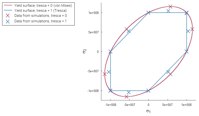
The principal stresses at termination are checked.
Tests
This benchmark is associated with 24 tests.
*MAT_MMC
Damage
"Optional title"
mid, $\rho$, $G$
$\sigma_c$, $\sigma_x$, $P_x$, $\sigma_{cap}$, $\alpha$, $\varepsilon_{p,fail}$, $yield$
$K$, $\beta$, $\varepsilon_{v,max}$, $c$, $\dot{\varepsilon}_0$, $\psi$, $d$, $d_{dec}$
Damage in *MAT_MMC is verified in this test.
Tested parameter: $\varepsilon_{p,fail}$
Two CHEX elements are used in this test. One of the elements is loaded in uniaxial tension and the other to uniaxial compression.
Effective stress vs. time and damage vs. effective plastic strain from both elements are presented in Figure 1 and 2 together with target curves from a verification script.
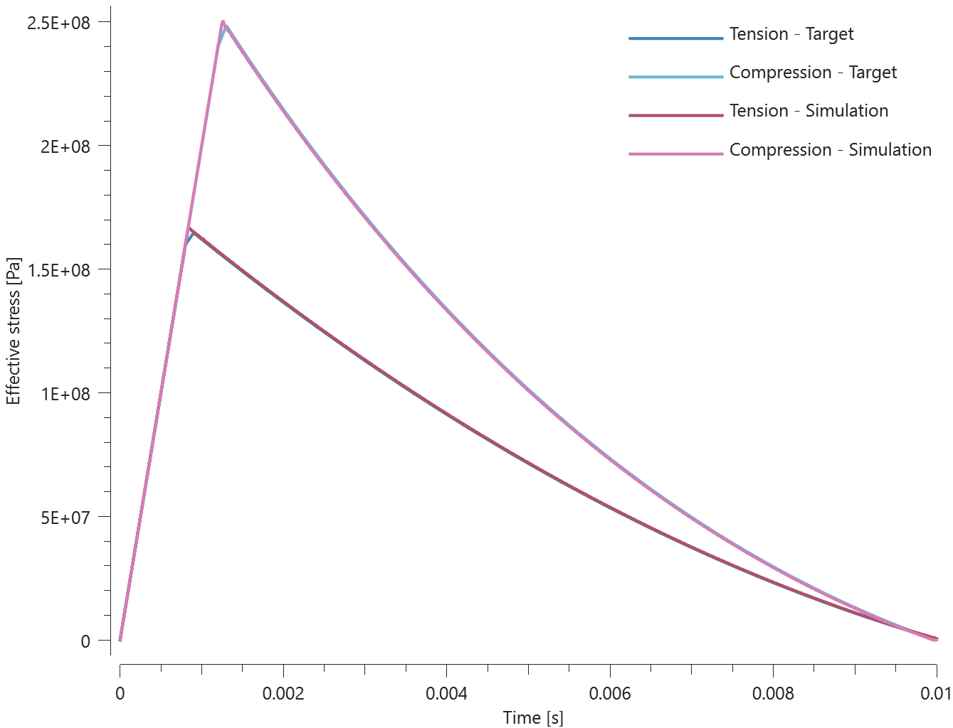
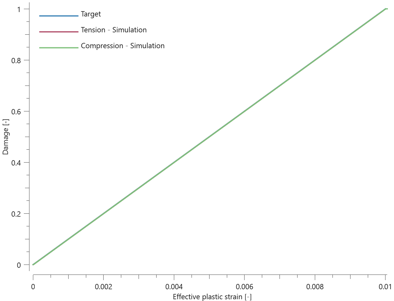
Maximum and average effective stress, effective plastic strain and damage are checked in both elements.
Tests
This benchmark is associated with 1 tests.
Direction of plastic flow and bulking cap
"Optional title"
mid, $\rho$, $G$
$\sigma_c$, $\sigma_x$, $P_x$, $\sigma_{cap}$, $\alpha$, $\varepsilon_{p,fail}$, $yield$
$K$, $\beta$, $\varepsilon_{v,max}$, $c$, $\dot{\varepsilon}_0$, $\psi$, $d$, $d_{dec}$
The bulking feature of *MAT_MMC is verified in this test.
Tested parameters: $\beta$ and $\varepsilon_{v,max}$.
Two CHEX elements are compressed in the Z-direction while fixed in the X- and Y-direciton. Bulking with a cap on the bulking strain is active in one of the elements.
Effective stress vs. pressure from both elements are presented in Figure 1 together with target curves from a verification script.
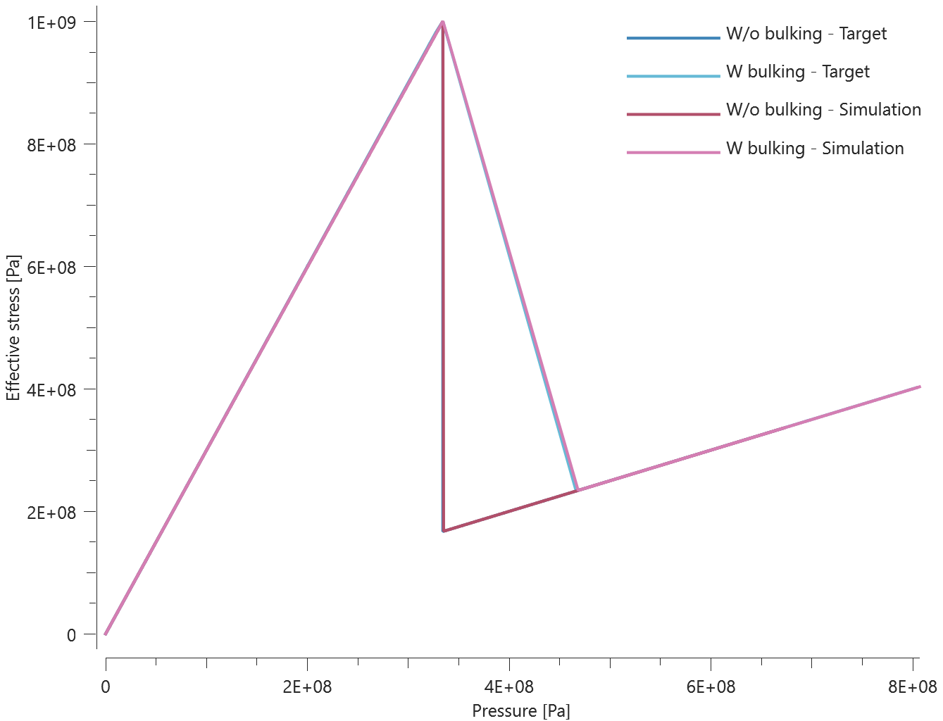
Maximum and average effective stress and pressure are checked for both elements. Maximum bulking strain is checked in the element with bulking activated and it should be equal to $\varepsilon_{v,max}$.
Tests
This benchmark is associated with 1 tests.
Strain rate effects
"Optional title"
mid, $\rho$, $G$
$\sigma_c$, $\sigma_x$, $P_x$, $\sigma_{cap}$, $\alpha$, $\varepsilon_{p,fail}$, $yield$
$K$, $\beta$, $\varepsilon_{v,max}$, $c$, $\dot{\varepsilon}_0$, $\psi$, $d$, $d_{dec}$
The strain rate effects in *MAT_MMC are verified in this test.
Tested parameters: $c$, $\dot{\varepsilon}_0$ and $\psi$.
The model consist of three sets of elements, with two elements in each set. One of the elements in each set is loaded in uniaxial compression and the other in uniaxial tension. The loading is caused by a prescribed strain rate.
In the first set of elements, no rate effects are included. In the second and third set, rate effects are included. In the second set, $\psi$ is set to 0.0 and in the third set, $\psi$ is set to $1.0$.
Effective stress vs. pressure at yield from the elements are presented in Figure 1 together with target curves of the yield strength vs. pressure.
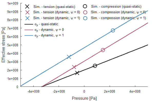
Maximum and average effective stress in the elements are checked.
Tests
This benchmark is associated with 3 tests.
Viscous damping
"Optional title"
mid, $\rho$, $G$
$\sigma_c$, $\sigma_x$, $P_x$, $\sigma_{cap}$, $\alpha$, $\varepsilon_{p,fail}$, $yield$
$K$, $\beta$, $\varepsilon_{v,max}$, $c$, $\dot{\varepsilon}_0$, $\psi$, $d$, $d_{dec}$
The viscous damping in *MAT_MMC is verified in this test.
Tested parameters: $d$ and $d_{dec}$.
Two CHEX elements are compressed in the Z-direction while fixed in the X- and Y-direction. The compression is done at a prescribed strain rate and damping is used in one of the elements.
Effective stress vs. time from the elements are presented in Figure 1 together with target curves from a verification script.
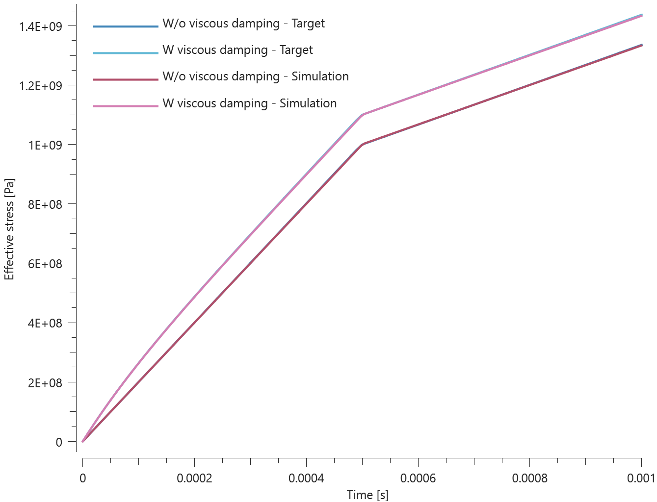
Maximum and average effective stress is checked for both elements.
Tests
This benchmark is associated with 1 tests.
Yield and failure surface
"Optional title"
mid, $\rho$, $G$
$\sigma_c$, $\sigma_x$, $P_x$, $\sigma_{cap}$, $\alpha$, $\varepsilon_{p,fail}$, $yield$
$K$, $\beta$, $\varepsilon_{v,max}$, $c$, $\dot{\varepsilon}_0$, $\psi$, $d$, $d_{dec}$
The yield surface and failure surface in *MAT_MMC are verified in this test.
Tested parameters: $\sigma_c$, $\sigma_x$, $P_x$, $\sigma_{cap}$, $\alpha$ and $yield$.
Four CHEX elements are used in this test, which is divided into two steps.
In step 1, two of the elements are loaded to confinement pressures P3 and P4.
In step 2, one of the elements is stretched while the others are compressed.
The loading continues until failure occurs in all elements. With the selected damage parameters, failure occurs as soon as the effective stress reaches the yield surface. The loading conditions for each of the elements are presented in Table 1.
| Element ID | Step 1, Confinement pressure | Step 2, Loading (uniaxial) |
|---|---|---|
| 1 | 0 | tension |
| 2 | 0 | compression |
| 3 | p3 | compression |
| 4 | p4 | compression |
The model is run with both von Mises and Rankine yield surface.
Effective stress vs. pressure prior to and post failure for the four elements in the von Mises model are presented in Figure 1, together with the yield and failure surfaces.
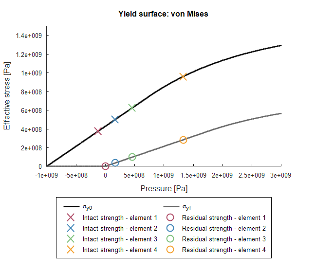
Effective stress vs. pressure prior to and post failure for the four elements in the Rankine model are presented in Figure 2, together with the yield and failure surfaces.
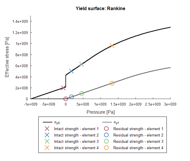
Maximum, minimum and average effective stress are checked in the elements.
Tests
This benchmark is associated with 4 tests.
*MAT_MMC_OST
Nonlinear pressure-volume relationship
"Optional title"
mid, $\rho_0$, $G$
$\sigma_c$, $\sigma_x$, $p_x$, $\sigma_{cap}$, $c_{1,f}$, $\sigma_{cap,f}$, $\varepsilon_{p,f}$, $s$
$K_1$, $K_2$, $K_3$, $yield$, $\beta$, $\varepsilon_{v,max}$, $c$, $\dot{\varepsilon}_0$,
$\psi$, $d$, $d_{dec}$, nsplit
The nonlinear pressure response in volumetric compression is verified in this test.
Tested parameters: $K_1$, $K_2$ and $K_3$.
A LHEX element is volumetrically compressed to a prescribed strain. The specified pressure-volume relationship incorporates a linear, a quadratic and a cubic term. Pressure vs. volumetric strain extracted from the model is presented in Figure 1 together with a target curve.
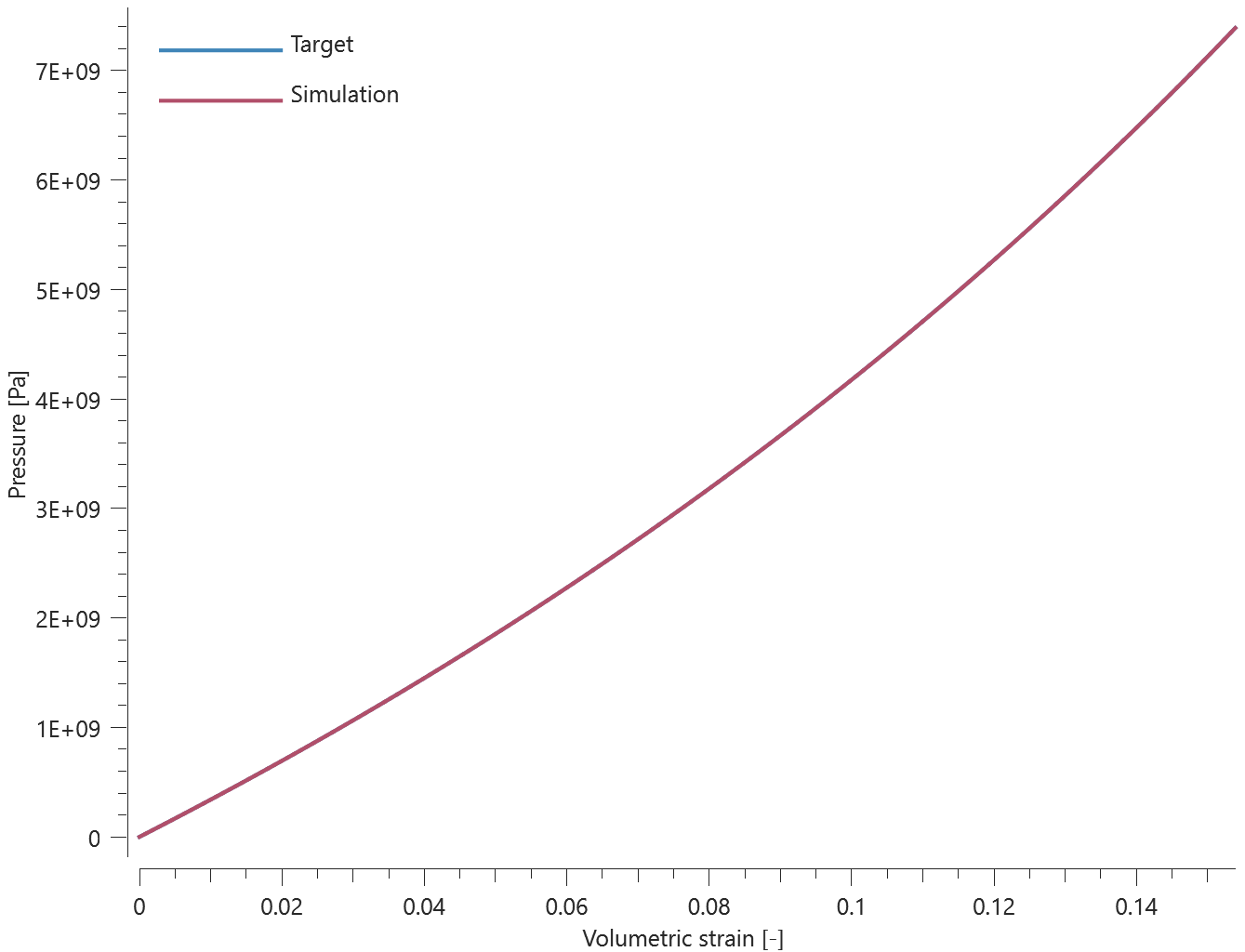
Maximum and average pressure are checked.
Tests
This benchmark is associated with 1 tests.
Nonlinear pressure-volume relationship - SPH
"Optional title"
mid, $\rho_0$, $G$
$\sigma_c$, $\sigma_x$, $p_x$, $\sigma_{cap}$, $c_{1,f}$, $\sigma_{cap,f}$, $\varepsilon_{p,f}$, $s$
$K_1$, $K_2$, $K_3$, $yield$, $\beta$, $\varepsilon_{v,max}$, $c$, $\dot{\varepsilon}_0$,
$\psi$, $d$, $d_{dec}$, nsplit
The nonlinear pressure response in volumetric compression is verified in this test.
Tested parameters: $K_1$, $K_2$ and $K_3$.
A cubic geometry filled with SPH-particles is volumetrically compressed to a prescribed pressure. The specified pressure-volume relationship incorporates a linear, a quadratic and a cubic term. Pressure vs. volumetric strain extracted from the model is presented in Figure 1 together with a target curve.
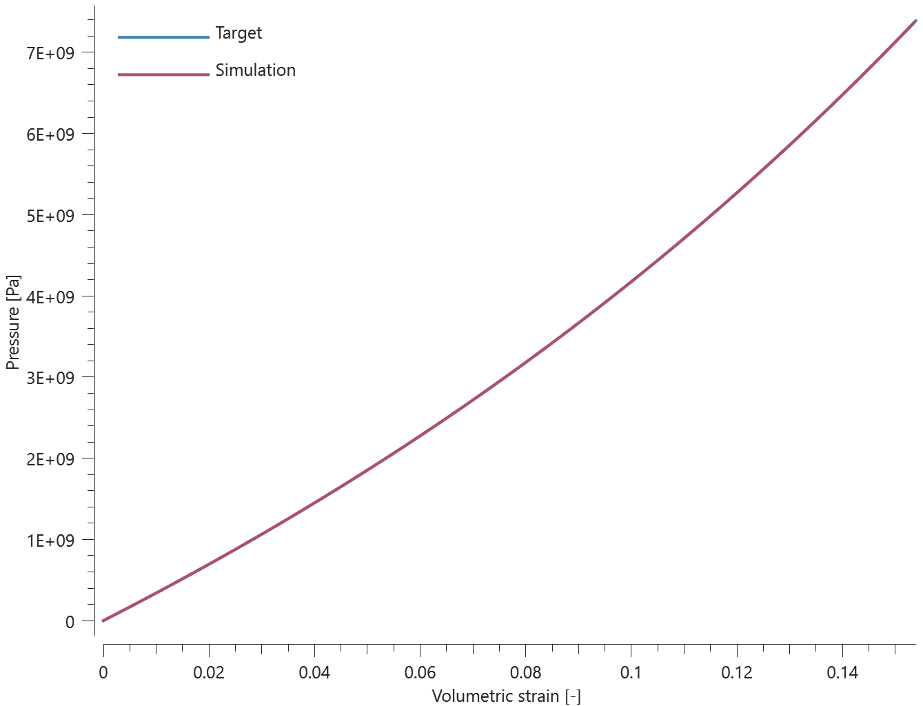
Maximum and average pressure are checked.
Tests
This benchmark is associated with 1 tests.
Quasi-static flow surface
"Optional title"
mid, $\rho_0$, $G$
$\sigma_c$, $\sigma_x$, $p_x$, $\sigma_{cap}$, $c_{1,f}$, $\sigma_{cap,f}$, $\varepsilon_{p,f}$, $s$
$K_1$, $K_2$, $K_3$, $yield$, $\beta$, $\varepsilon_{v,max}$, $c$, $\dot{\varepsilon}_0$,
$\psi$, $d$, $d_{dec}$, nsplit
The quasi-static yield and residual surface is verified in this test.
Tested parameters: $\sigma_c$, $\sigma_x$, $p_x$, $\sigma_{cap}$ and $\varepsilon_{p,f}$.
Three elements are subjected to different loading conditions. The first element is stretched in the X-direction by a prescribed motion while unconstrained in the Y- and Z-direction, meaning that the element is subjected to a state of uniaxial tension. The second element is compressed instead of stretched, leading to a state of uniaxial compression. The third element is subjected to a confinement pressure of 500 MPa prior to being compressed in the X-direction. For all elements, the deformation in the X-direction continues until fracture occurs. Effective stress vs. pressure extracted from the elements is shown in Figure 1 together with the yield surface and the residual surface.
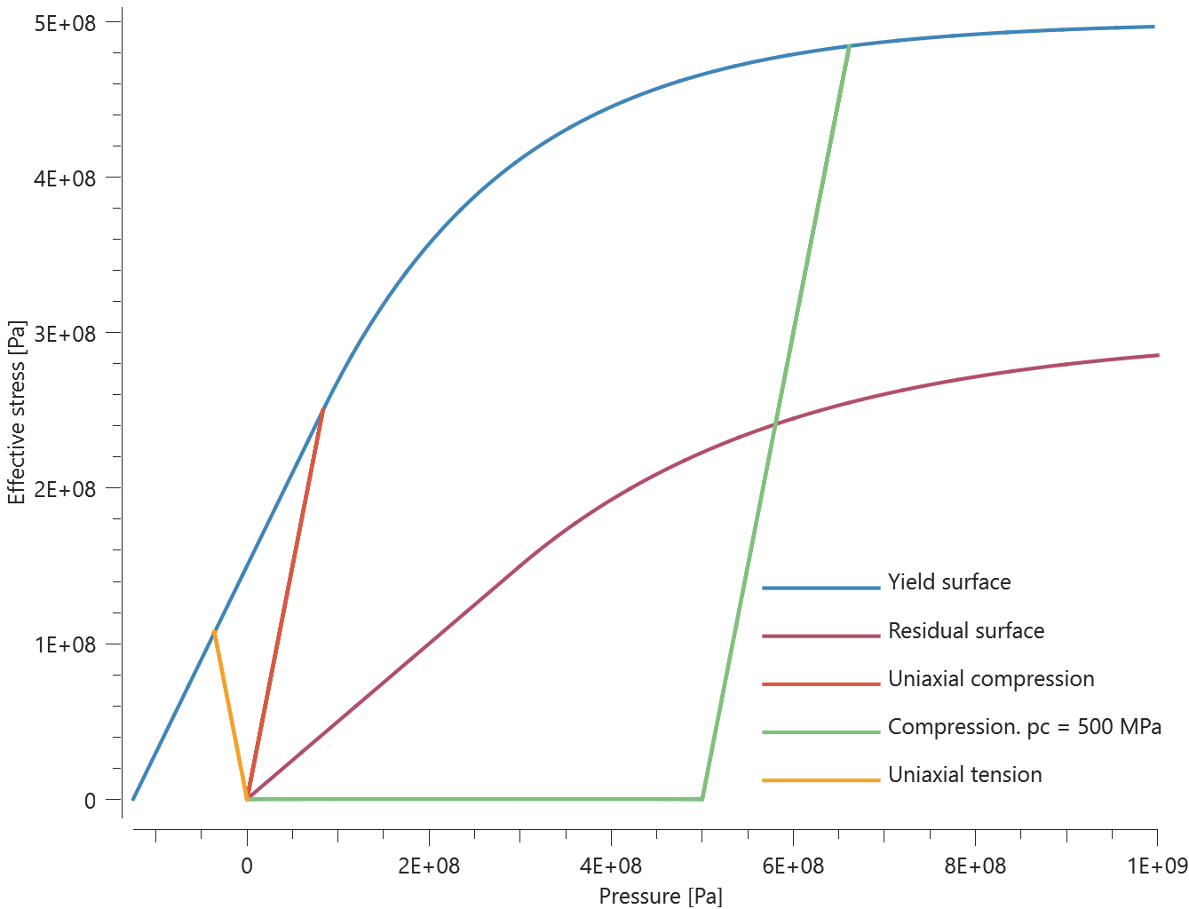
Effective stress vs. effective plastic strain extracted from the three elements are presented in Figures 2 - 4 below. The target curves included in the figures are obtained from another numerical approach.


Maximum and average values of effective stress, pressure and effective plastic strain are checked.
Tests
This benchmark is associated with 3 tests.
Strain rate effects and damping
"Optional title"
mid, $\rho_0$, $G$
$\sigma_c$, $\sigma_x$, $p_x$, $\sigma_{cap}$, $c_{1,f}$, $\sigma_{cap,f}$, $\varepsilon_{p,f}$, $s$
$K_1$, $K_2$, $K_3$, $yield$, $\beta$, $\varepsilon_{v,max}$, $c$, $\dot{\varepsilon}_0$,
$\psi$, $d$, $d_{dec}$, nsplit
Strain rate dependent yield surface is verified in this test.
Tested parameters: $c$, $\dot{\varepsilon}_0$, $\psi$ and $d$.
This test is configured as the test “Quasi-static flow surface” but with strain rate effects and damping incorporated. Effective stress vs. effective plastic strain extracted from the three elements are presented in Figures 6 - 8 below. The target curves included in the figures are obtained from another numerical approach.
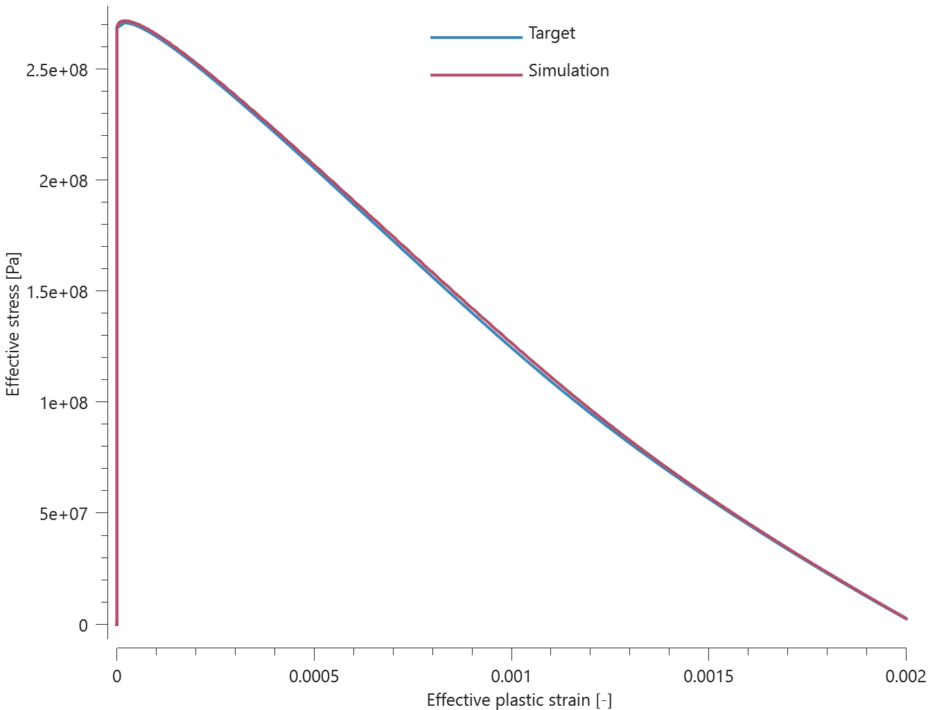


Maximum and average values of effective stress, pressure and effective plastic strain are checked.
Tests
This benchmark is associated with 3 tests.
Uniaxial strengths - SPH
"Optional title"
mid, $\rho_0$, $G$
$\sigma_c$, $\sigma_x$, $p_x$, $\sigma_{cap}$, $c_{1,f}$, $\sigma_{cap,f}$, $\varepsilon_{p,f}$, $s$
$K_1$, $K_2$, $K_3$, $yield$, $\beta$, $\varepsilon_{v,max}$, $c$, $\dot{\varepsilon}_0$,
$\psi$, $d$, $d_{dec}$, nsplit
The uniaxial compressive strength and the uniaxial tensile strength are verified in this test.
Tested parameters: $\sigma_c$, $\sigma_x$ and $p_x$.
The test consists of two cubic geometries filled with SPH-particles. One of the geometries is stretched and the other is compressed by prescribed motions in the X-direction. Orthogonal directions are unconstrained. The prescribed motions continue until the yield surface is reached. The compressive stress at termination should be equal to $\sigma_c$, see Figure 1.
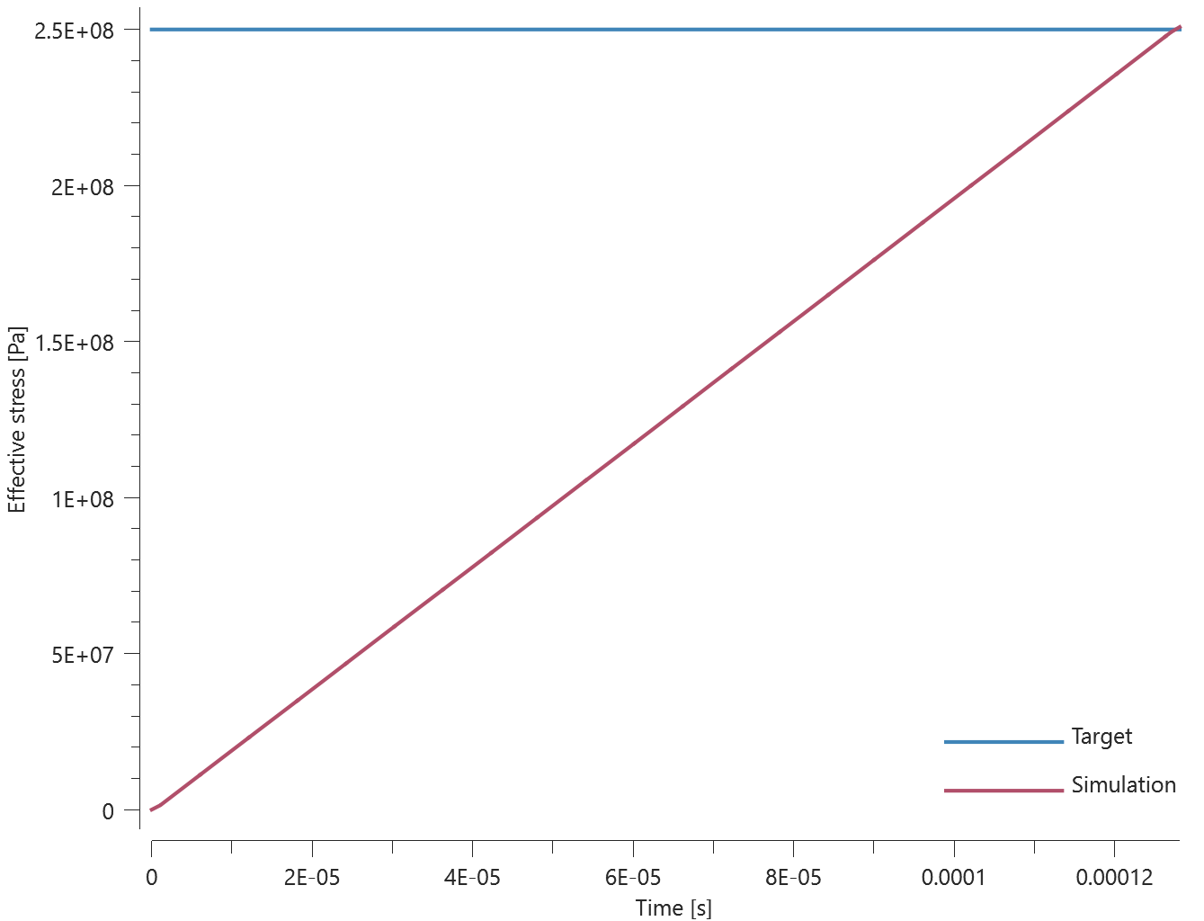
The tensile stress at termination should be equal to $\sigma_x$ (since $p_x$=-$\sigma_x$/3), see Figure 2.
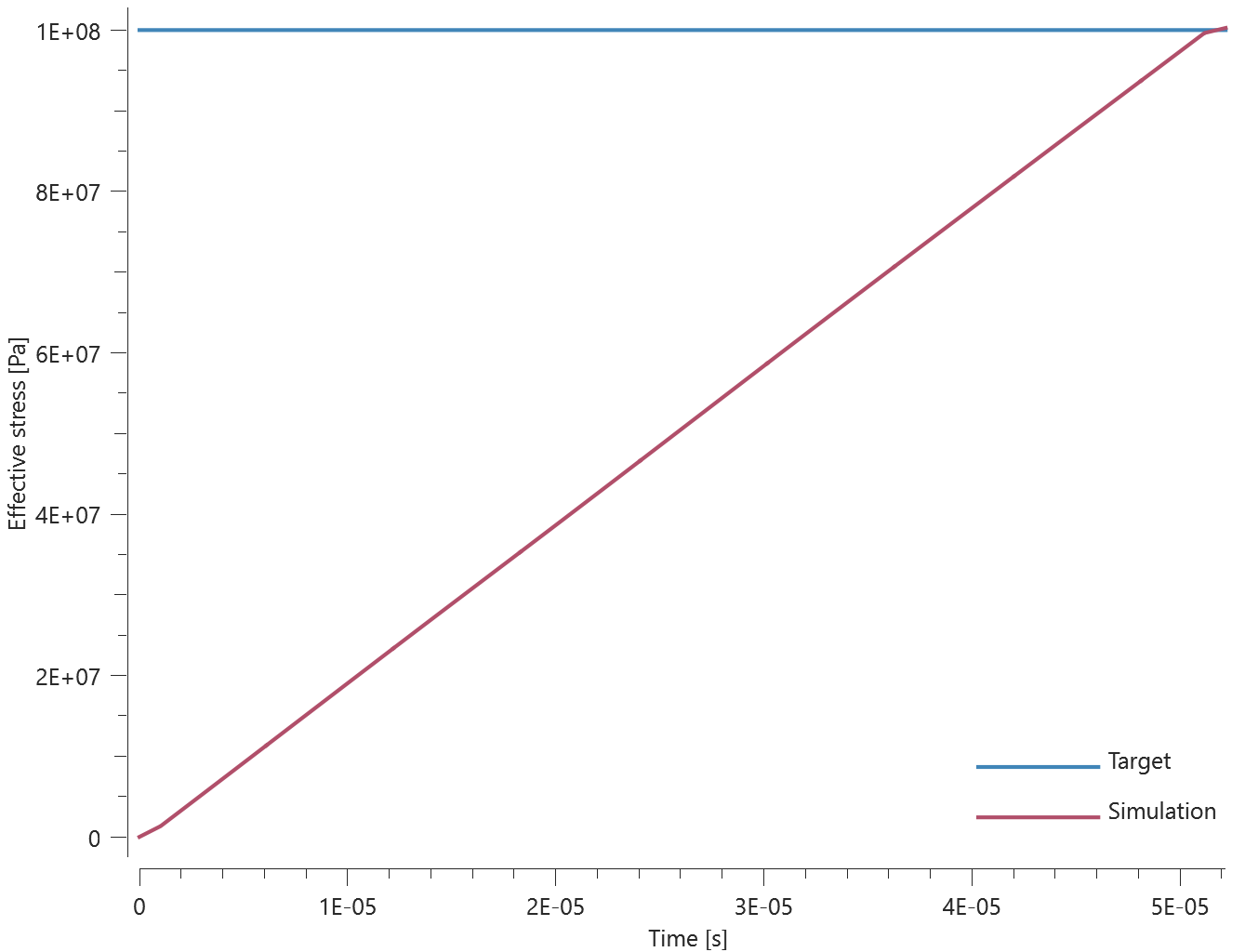
Last and average effective stress are checked.
Tests
This benchmark is associated with 2 tests.
*MAT_MM_CERAMIC - Bulking SPH
"Optional title"
mid, $\rho$, $G$
$\sigma_c$, $\sigma_x$, $P_x$, $\sigma_{cap}$, $\alpha$, $\varepsilon_{p,fail}$, yield
$K$, $\beta$, $\varepsilon_{v,max}$, $c$, $\dot{\varepsilon}_0$, $\psi$, $d$, $d_{dec}$
Tested parameters: $\beta$, $\varepsilon_{v,max}$.
Aside from the inclusion of bulking, the model parameters remain identical to those used in the test of the quasi-static response (compression only).
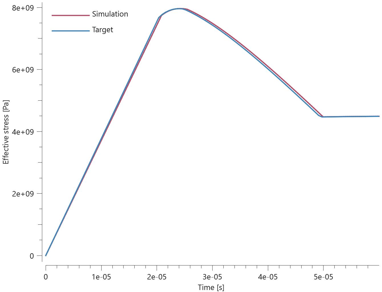
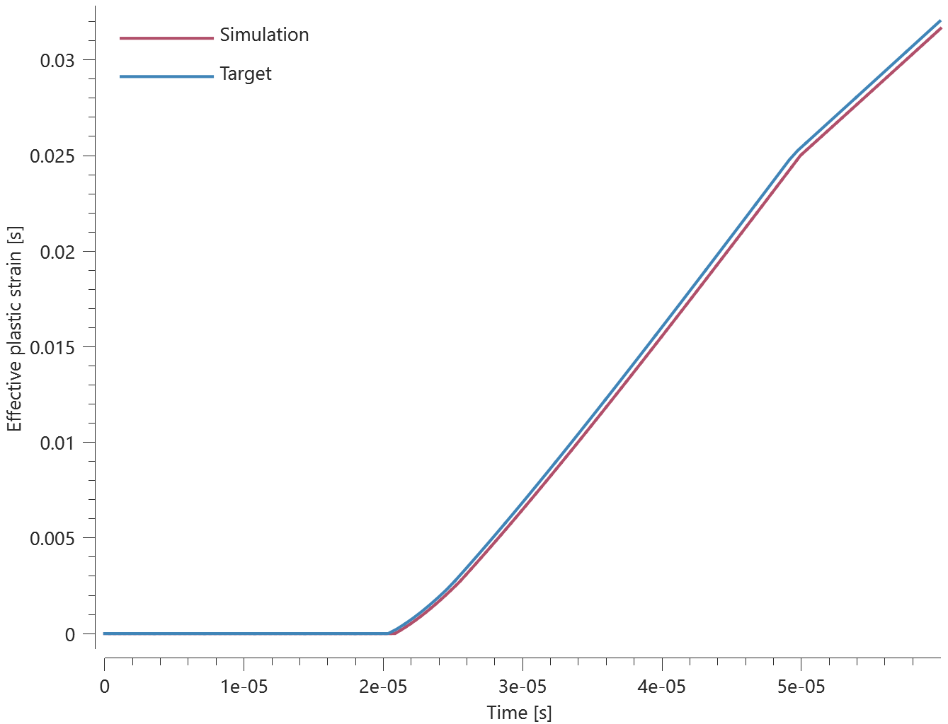
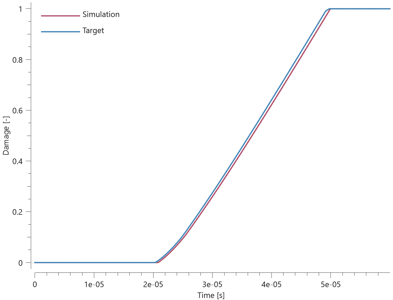
Maximum, average and last values of effective stress, effective plastic strain and damage are checked for version control.
Tests
This benchmark is associated with 1 tests.
*MAT_MM_CERAMIC - Dynamic response SPH
"Optional title"
mid, $\rho$, $G$
$\sigma_c$, $\sigma_x$, $P_x$, $\sigma_{cap}$, $\alpha$, $\varepsilon_{p,fail}$, yield
$K$, $\beta$, $\varepsilon_{v,max}$, $c$, $\dot{\varepsilon}_0$, $\psi$, $d$, $d_{dec}$
Tested parameters: $c$, $\dot{\varepsilon}_0$ and $\psi$.
Aside from the inclusion of strain rate hardening, the model parameters remain identical to those used in the test of the quasi-static response.
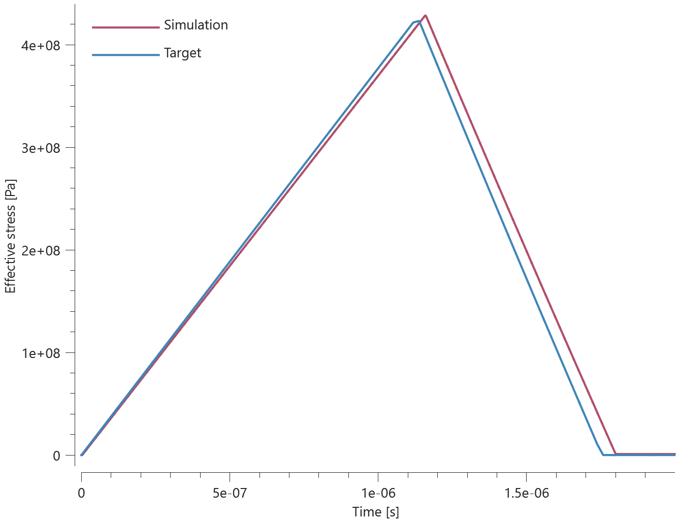
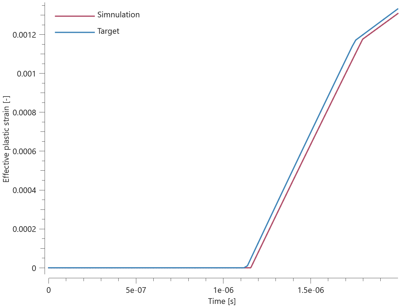
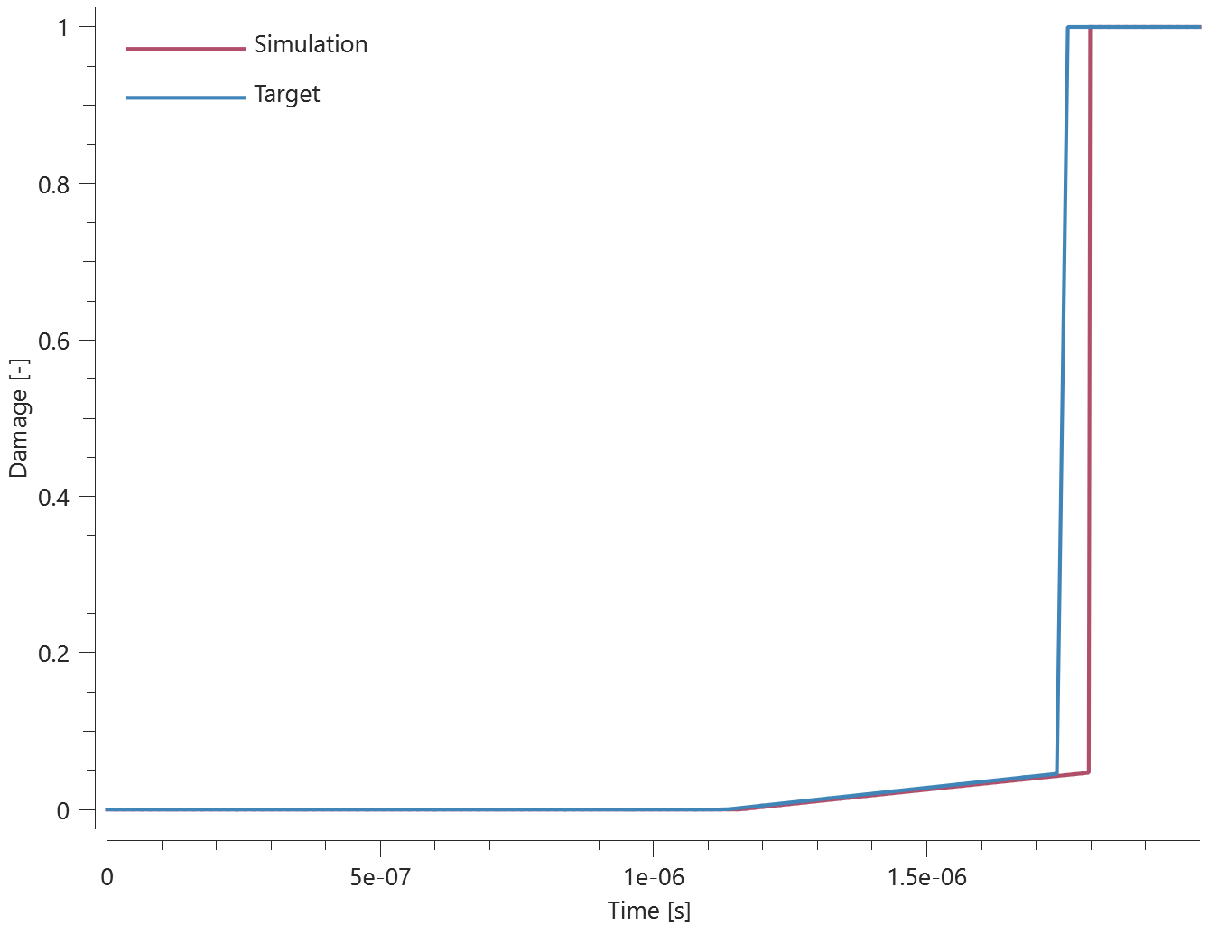
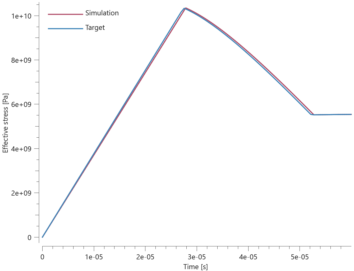
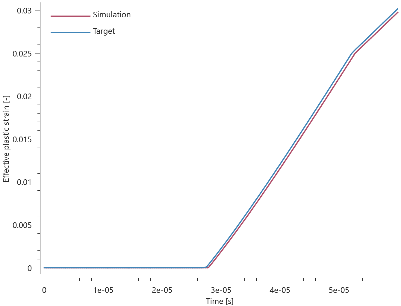
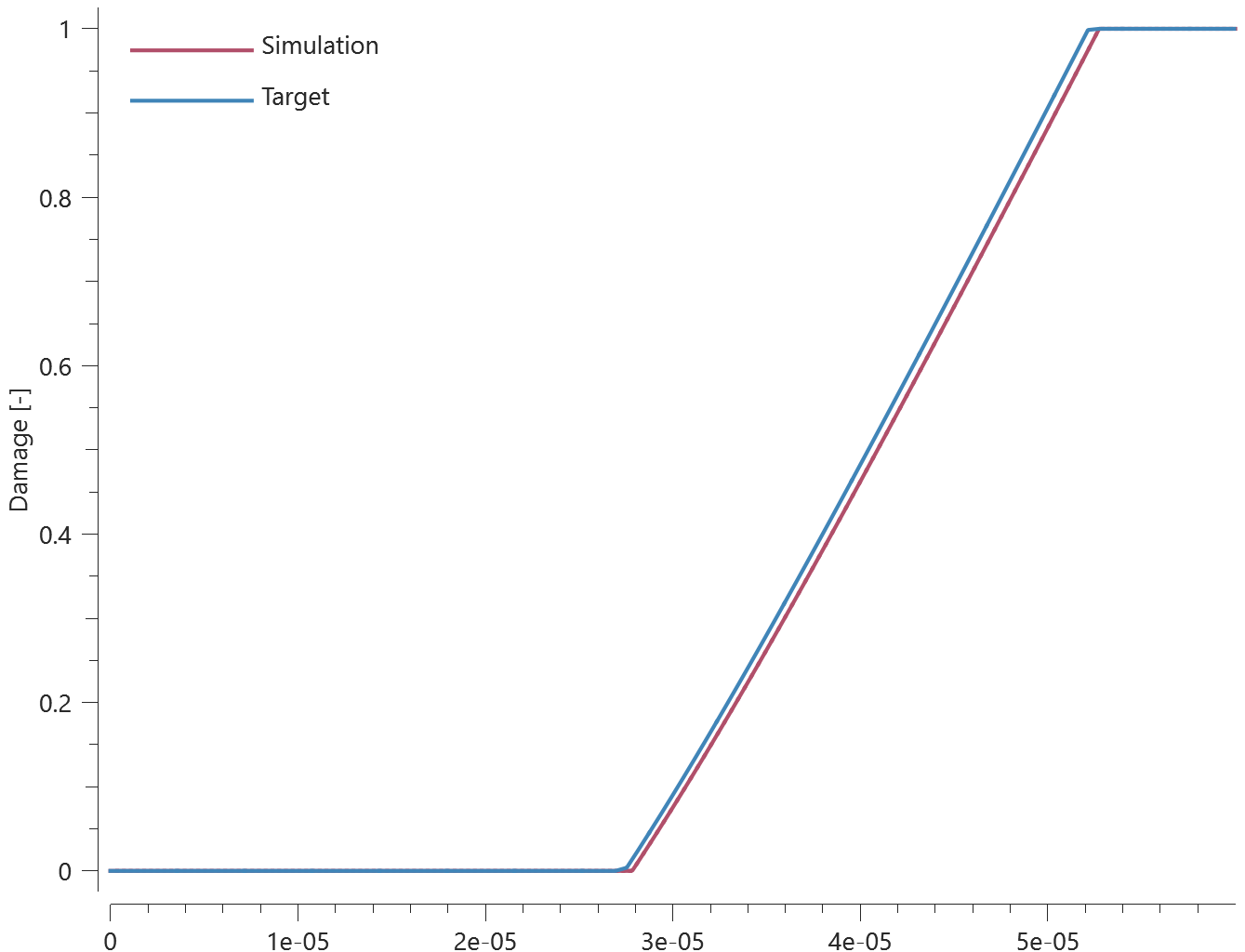
Maximum, average and last values of effective stress, effective plastic strain and damage are checked for version control.
Tests
This benchmark is associated with 2 tests.
*MAT_MM_CERAMIC - Quasi-static response SPH
"Optional title"
mid, $\rho$, $G$
$\sigma_c$, $\sigma_x$, $P_x$, $\sigma_{cap}$, $\alpha$, $\varepsilon_{p,fail}$, yield
$K$, $\beta$, $\varepsilon_{v,max}$, $c$, $\dot{\varepsilon}_0$, $\psi$, $d$, $d_{dec}$
Tested parameters: $G$,$\sigma_c$, $\sigma_x$,$P_x$, $\sigma_{cap}$, $\alpha$, $\varepsilon_{p,fail}$ and $K$.
A prescribed uniaxial strain rate, inducing either expansion or compression, is applied to a cube modeled using either FE or SPH. Effective stress, effective plastic strain and damage from the simulations are plotted in Figures 1 - 6 together with target curves obtained from a separate verification script. Strain rate hardening and bulking are not included in this test.
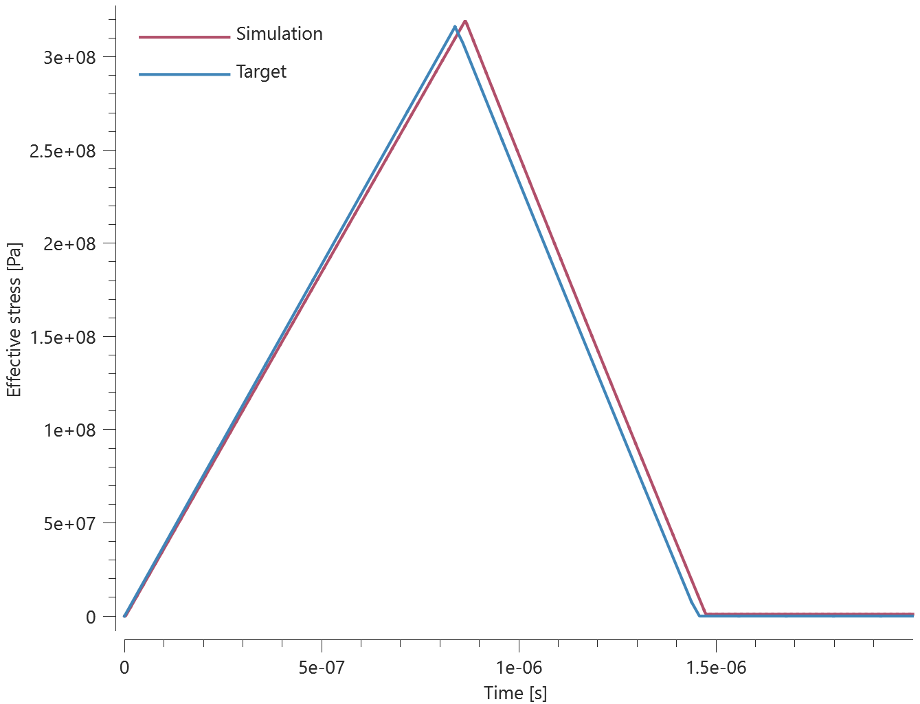
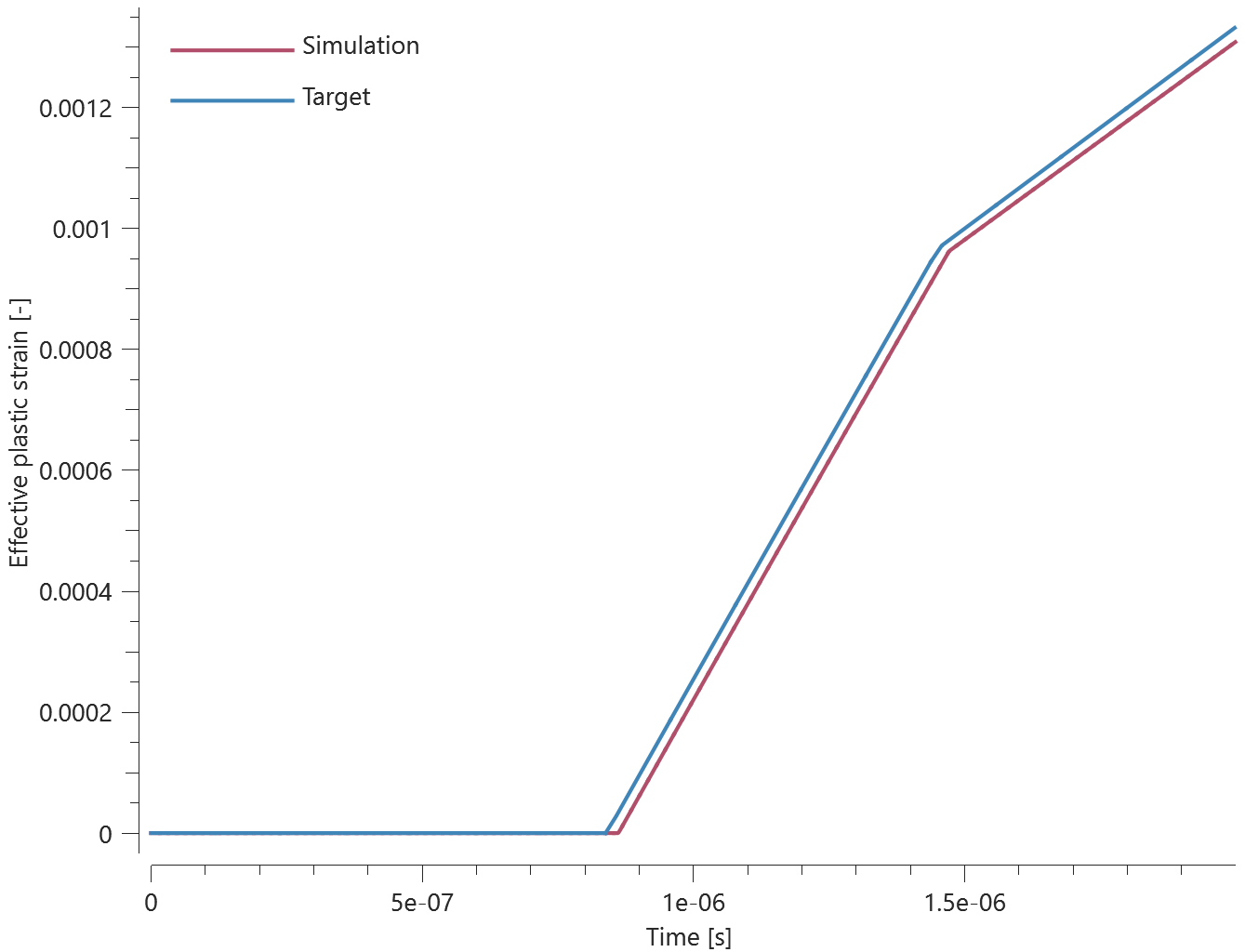
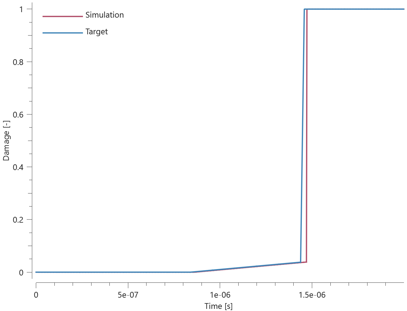
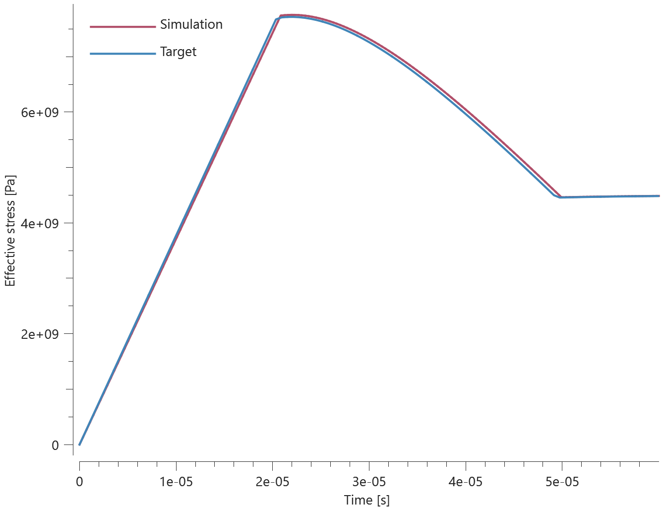

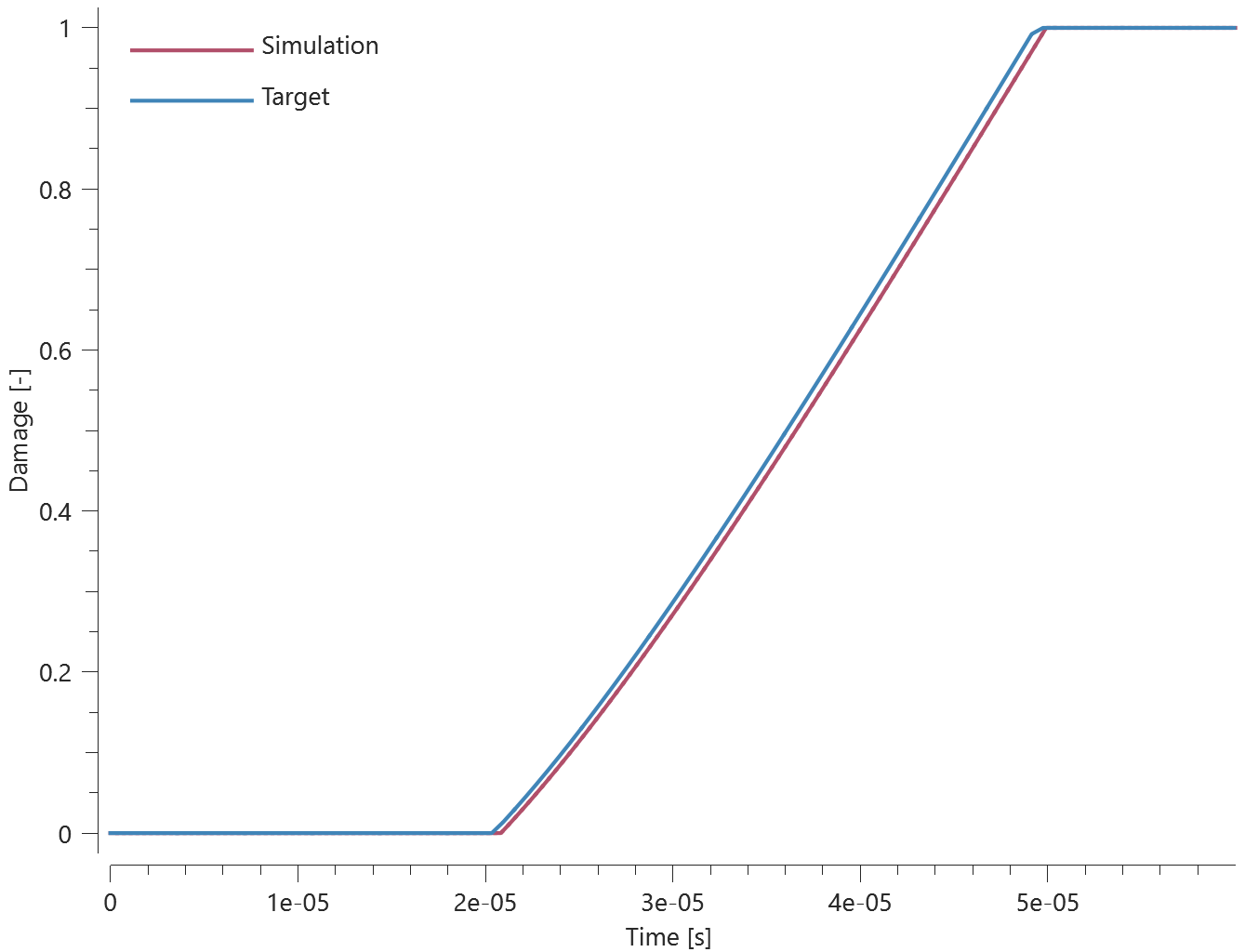
Maximum, average and last values of effective stress, effective plastic strain and damage are checked for version control.
Tests
This benchmark is associated with 2 tests.
*MAT_MM_CONCRETE
Elements subjected to a variety of stress states
"Optional title"
mid, $\rho$, $G$
$K_0$, $K_L$, $cid_{cmp}$, $f_t$, $f_c$, $\xi$, $\lambda$, $\gamma$
$\xi_y$, $\xi_r$, $\varepsilon_{p,u0}$, $\varepsilon_{p,r0}$, $\psi_p$, $\psi_r$, $\varepsilon_{p,u}^{min}$, $\varepsilon_{p,r}^{min}$
$m$, $bulk$, $bulk_{cap}$, $cid_{src}$, $cid_{srt}$, $c$, $\sigma_{y,min}$, $\sigma_{y,max}$
$\mu$, $G_{r0}$, $L_{ref}$, $nsplit$
Tested parameters: $G$, $K_{0}$, $K_{L}$, $cid_{cmp}$, $f_{t}$, $f_{c}$, $\xi$, $\lambda$, $\gamma$, $\xi_{y}$, $\xi_{r}$, $\varepsilon_{p,u0}$, $\varepsilon_{p,r0}$, $\psi_{p}$, $m$, $cid_{src}$, $cid_{srt}$, $G_{r0}$ and $L_{ref}$
Verification is done using a single LHEX element with generic material parameters. Fourteen different load cases are investigated, as presented in Table 1.
| Test | Confinement pressure [Mpa] | Subsequent deformation | Strain rate effects |
|---|---|---|---|
| 1 | 0 | compression | Excluded |
| 2 | 15 | compression | Excluded |
| 3 | 50 | compression | Excluded |
| 4 | 0 | Stretch | Excluded |
| 5 | 15 | Stretch | Excluded |
| 6 | 50 | Stretch | Excluded |
| 7 | 2000 | - | Excluded |
| 8 | 0 | compression | Included |
| 9 | 15 | compression | Included |
| 10 | 50 | compression | Included |
| 11 | 0 | Stretch | Included |
| 12 | 15 | Stretch | Included |
| 13 | 50 | Stretch | Included |
| 14 | 2000 | - | Included |
The confinement pressure is smoothly ramped up to the value specified in Table 1 and kept constant once reached. A subsequent deformation is imposed in all tests except Tests 5 and 12. The element is compressed or stretched by a constant velocity in the X-direction, while free to expand/contract in the orthogonal directions. The compression/stretching continues until the damage level equals 1. Strain rate effects are included in Tests 8 – 14.
Loading path to the initial yield surface for each test is illustrated in Figure 1. Note that the yield strength is not symmetric across the pressure axis, which is due to a defined lode parameter dependency.
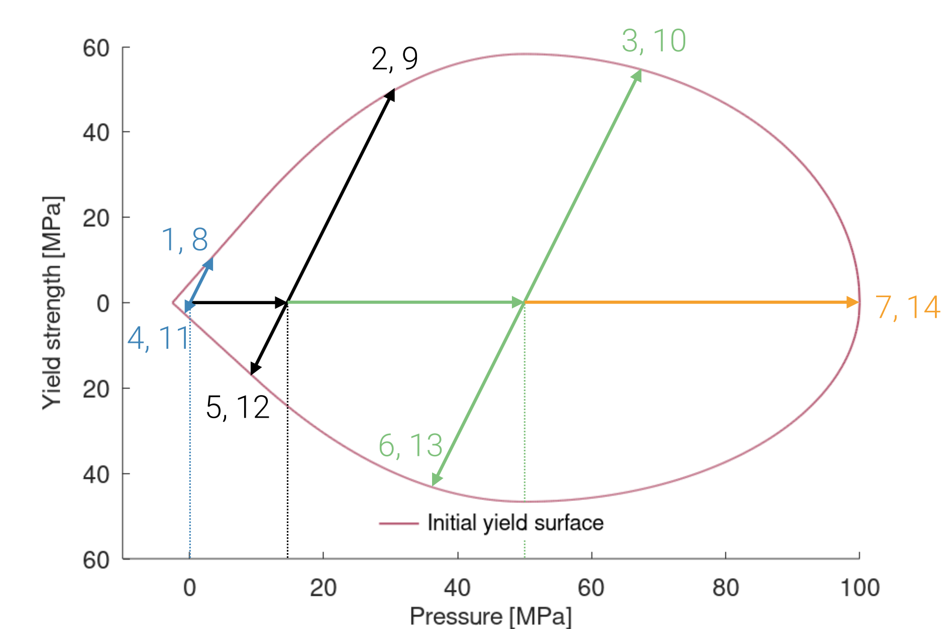
The curves presented below are extracted from simulations and compared to target curves obtained from an octave script.
Tests 1-6 and 8-13:
- Effective stress vs. effective plastic strain
- Damage vs. effective plastic strain
- Effective stress vs. pressure
Tests 7 and 14:
- Pressure vs. inelastic compaction
- Damage vs. inelastic compaction
- Effective stress vs. pressure
Test 1 - Quasi-static, uniaxial compression
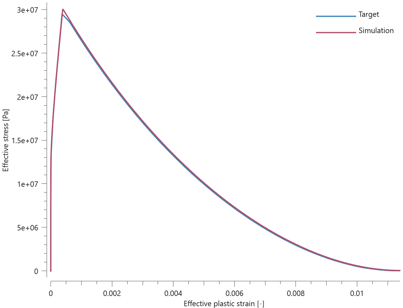
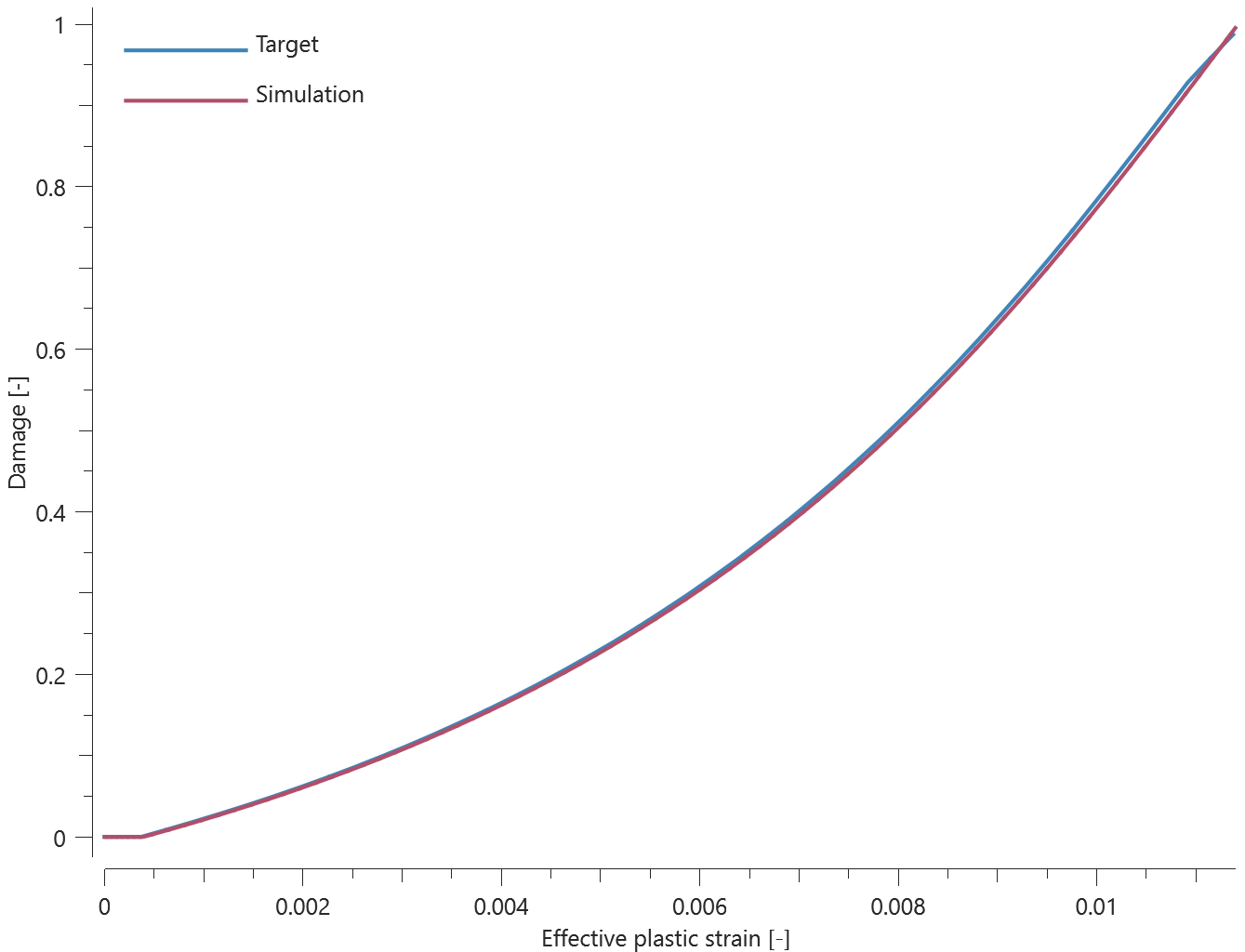
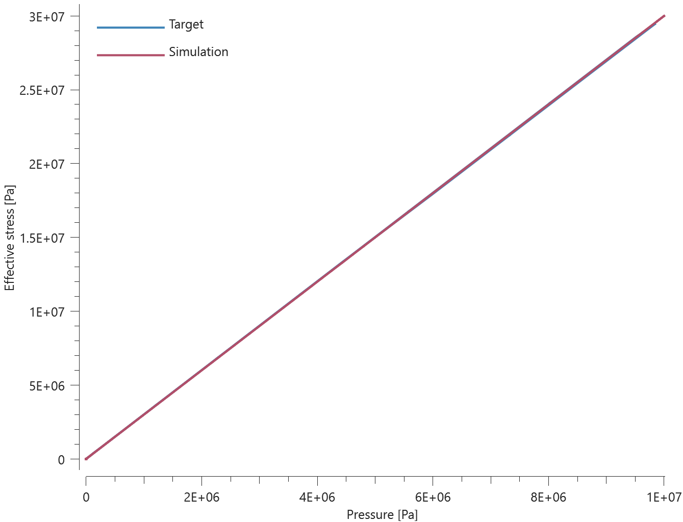
Test 2 - Quasi-static, compression at 15 MPa confinement pressure
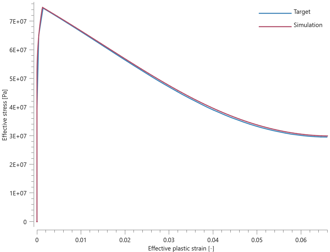

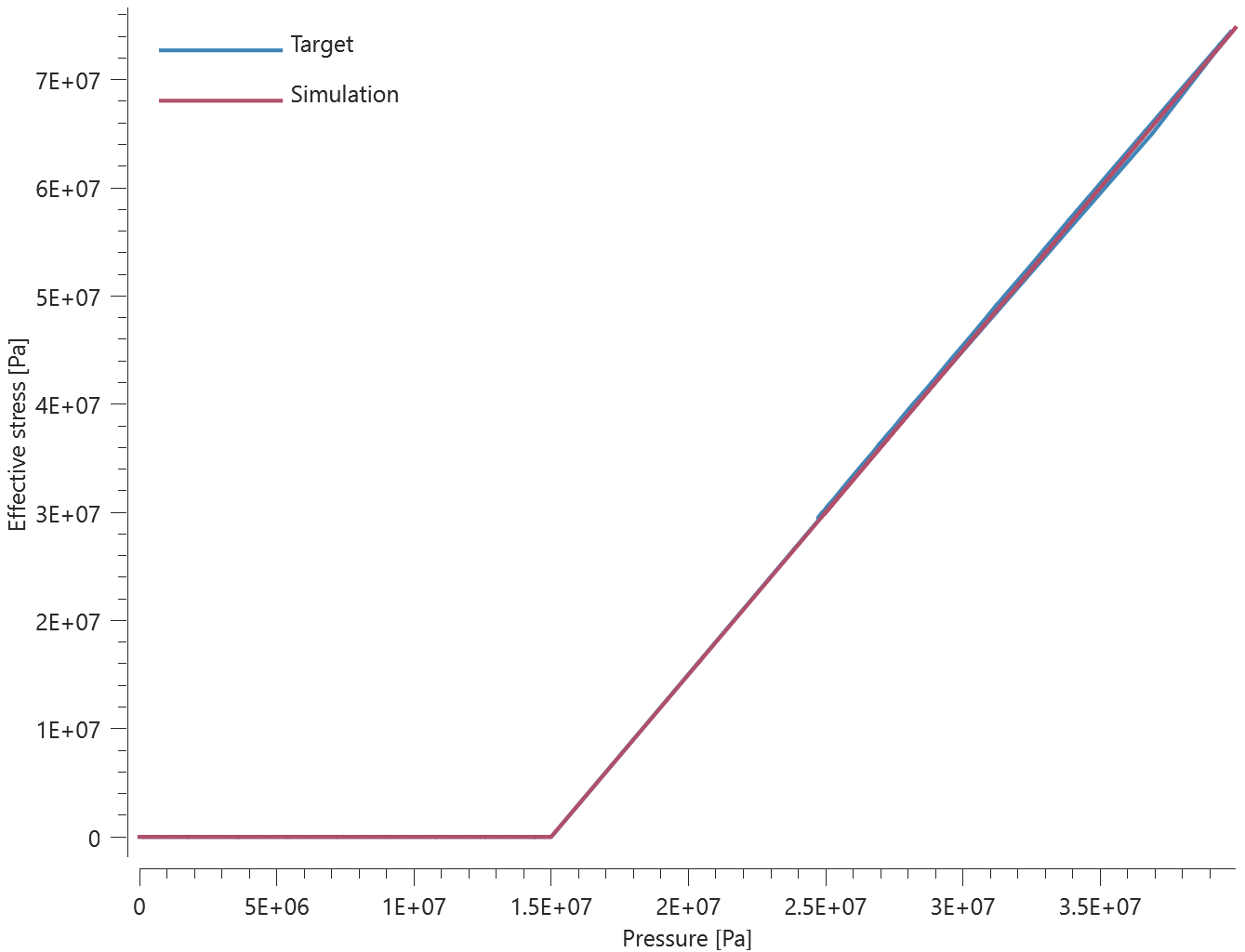
Test 3 - Quasi-static, compression at 50 MPa confinement pressure
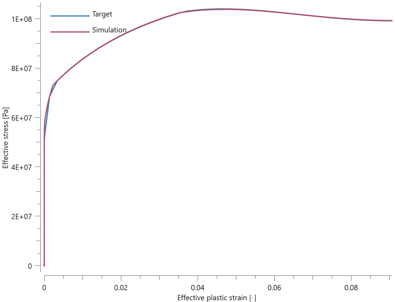

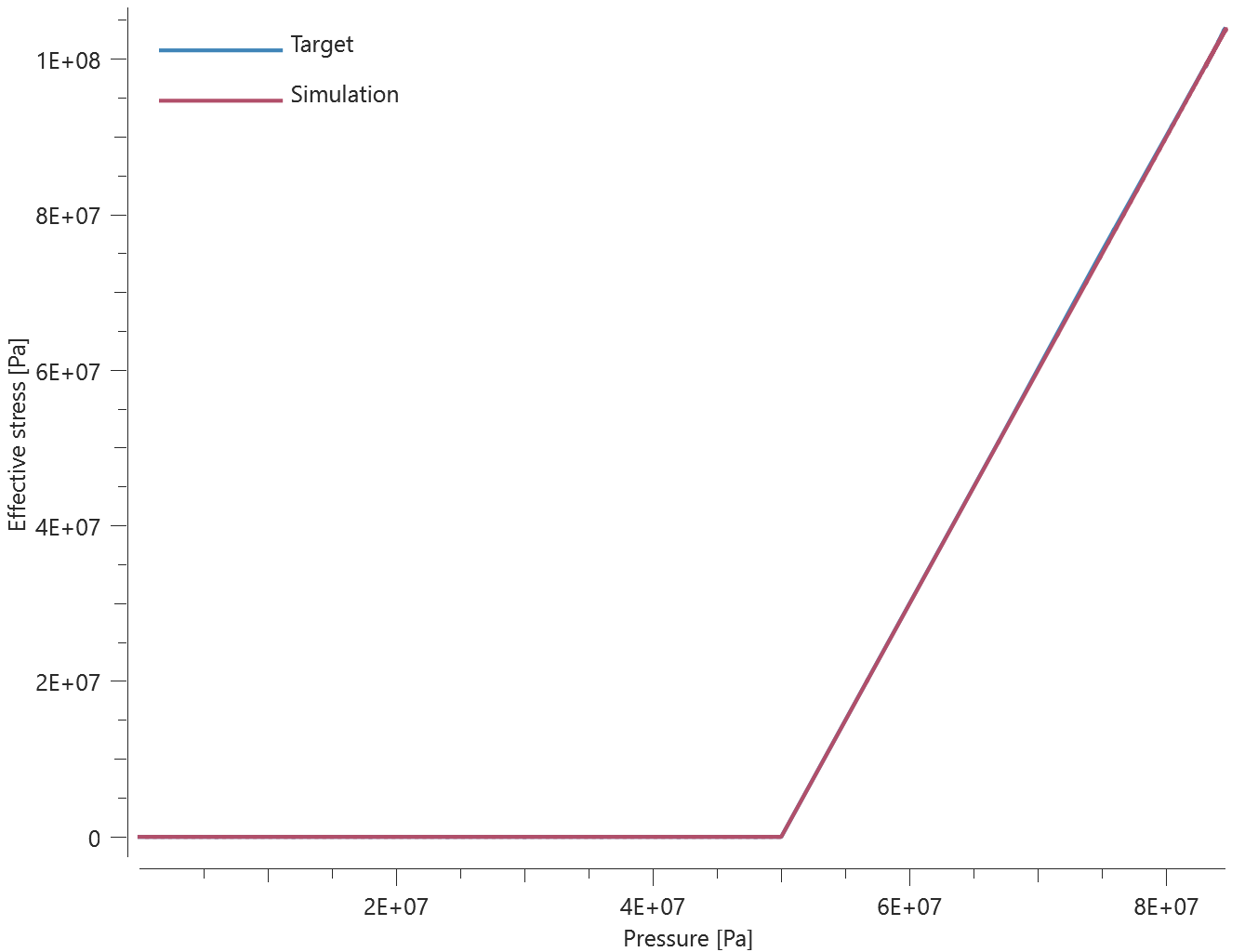
Test 4 - Quasi-static, uniaxial tension
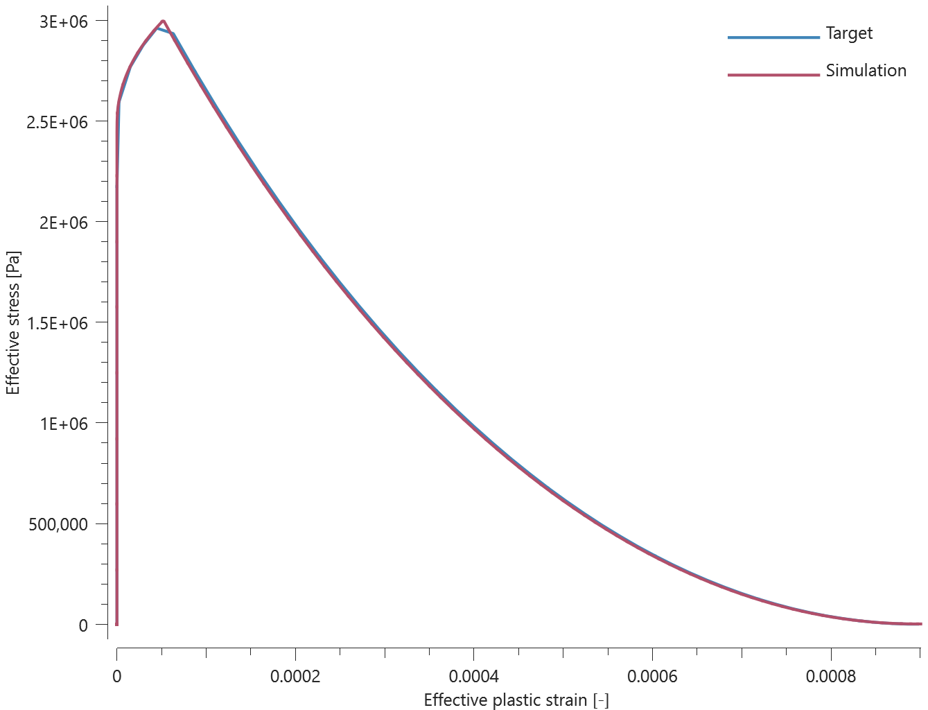
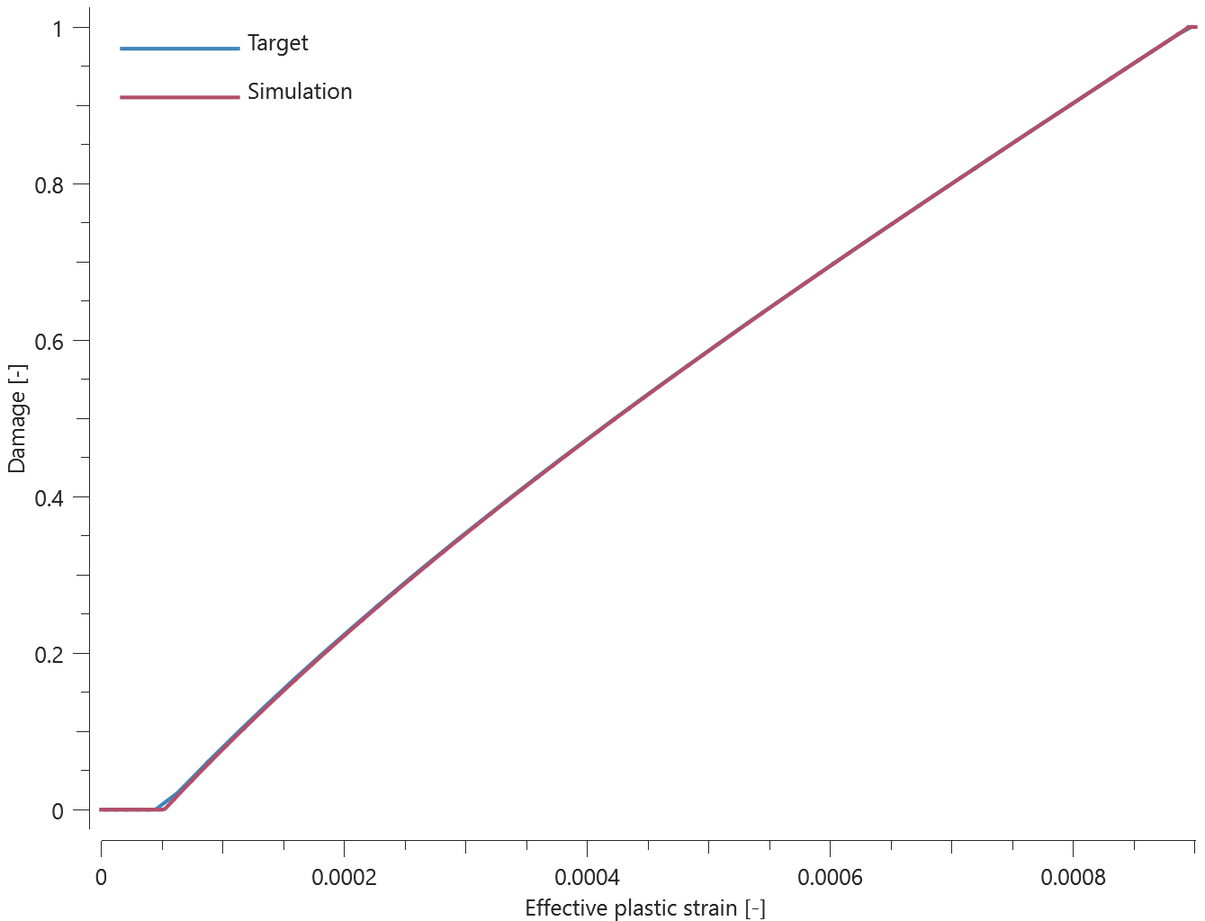
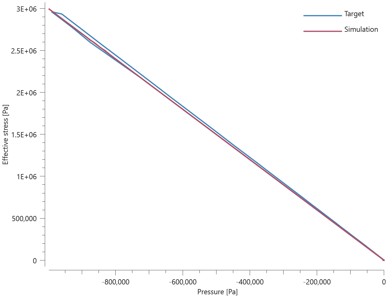
Test 5 - Quasi-static, stretching at 15 MPa confinement pressure
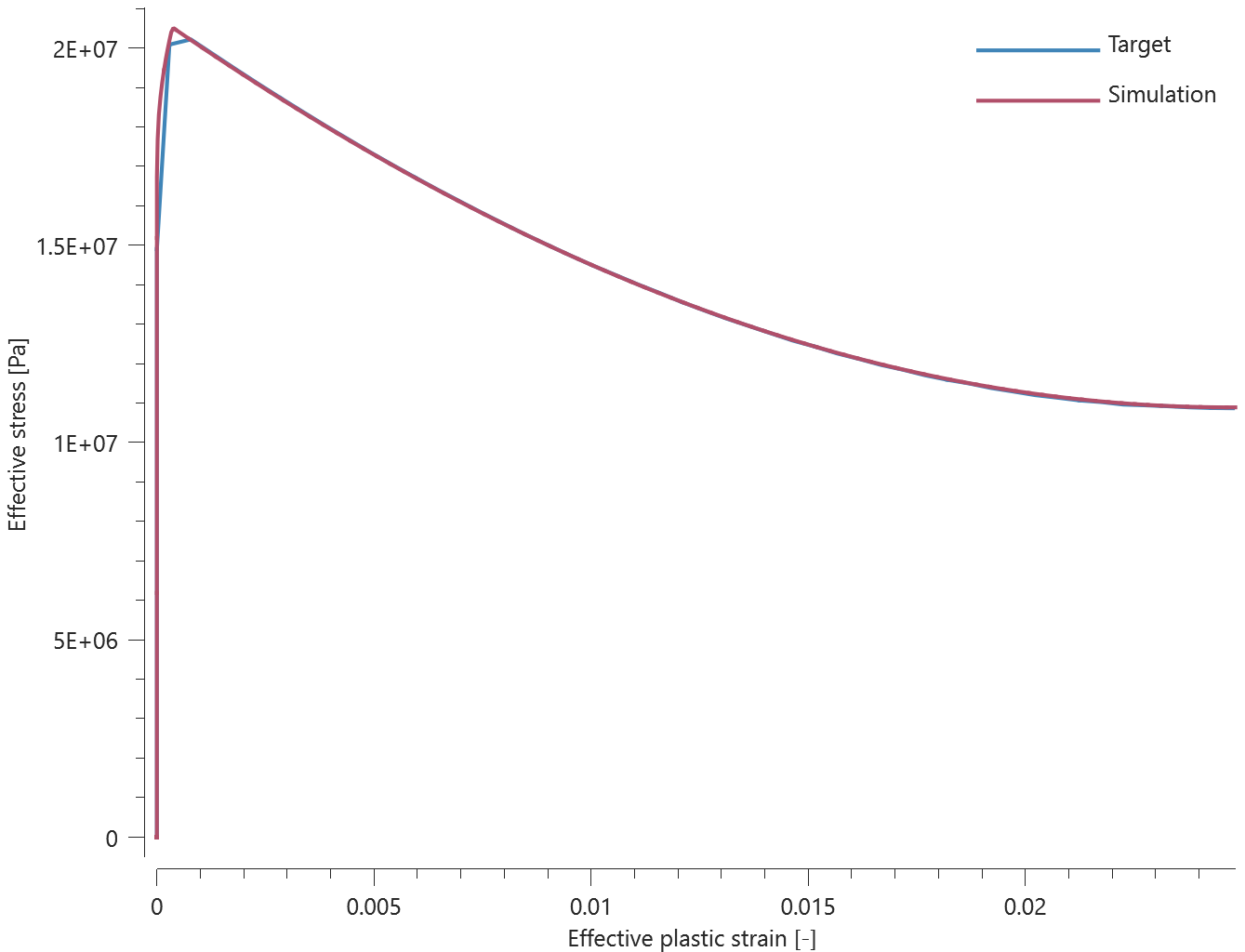
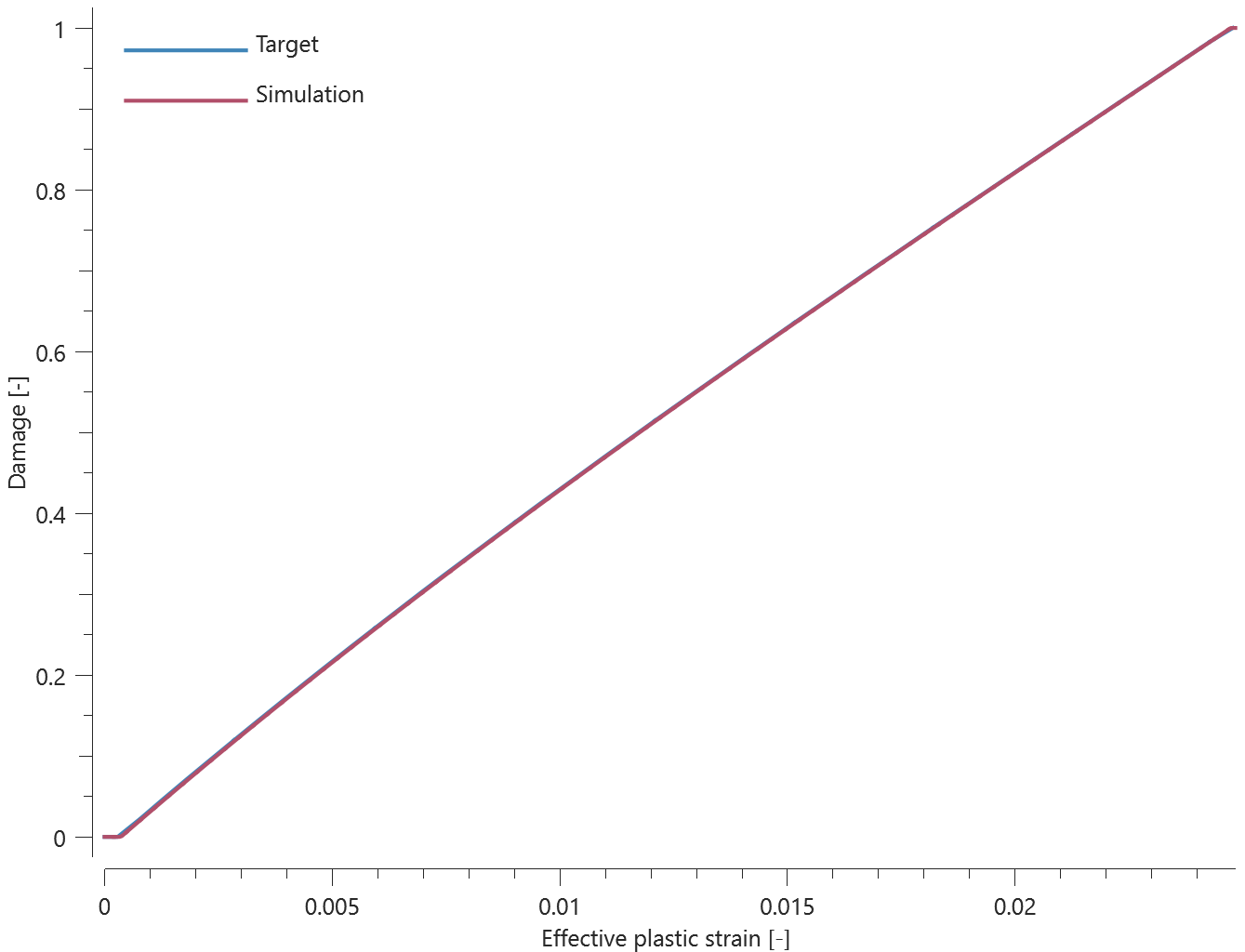
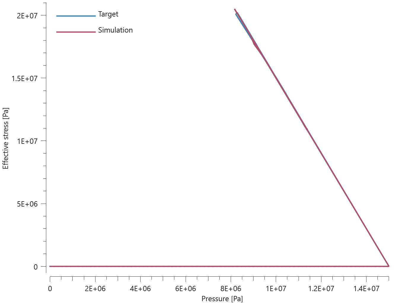
Test 6 - Quasi-static, stretching at 50 MPa confinement pressure
Test 7 - Quasi-static, volumetric compression

Test 8 - Dynamic, uniaxial compression
Test 9 - Dynamic, compression at 15 MPa confinement pressure
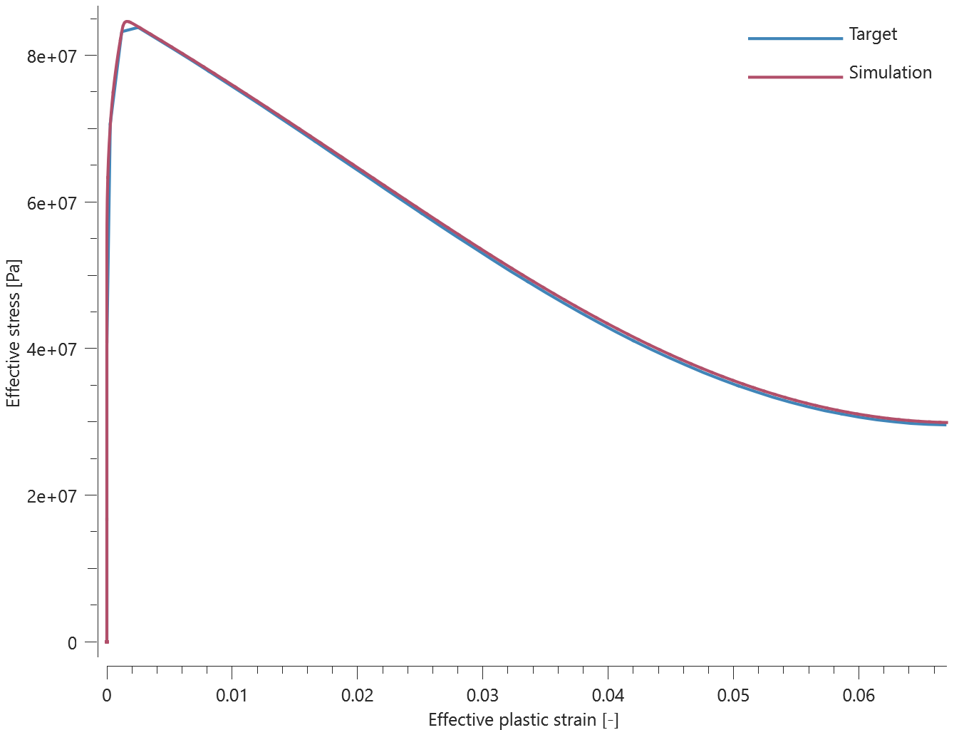

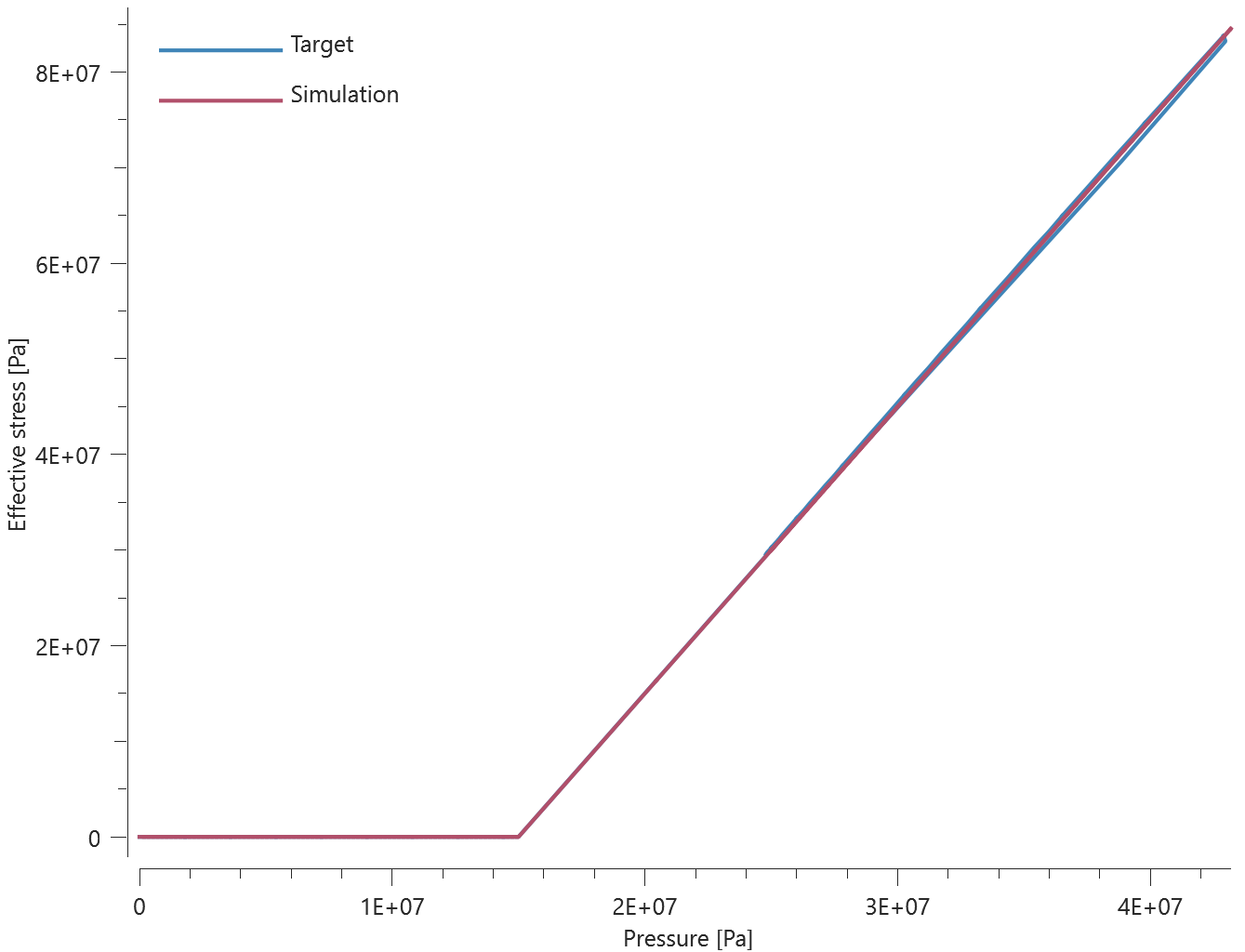
Test 10 - Dynamic, compression at 50 MPa confinement pressure
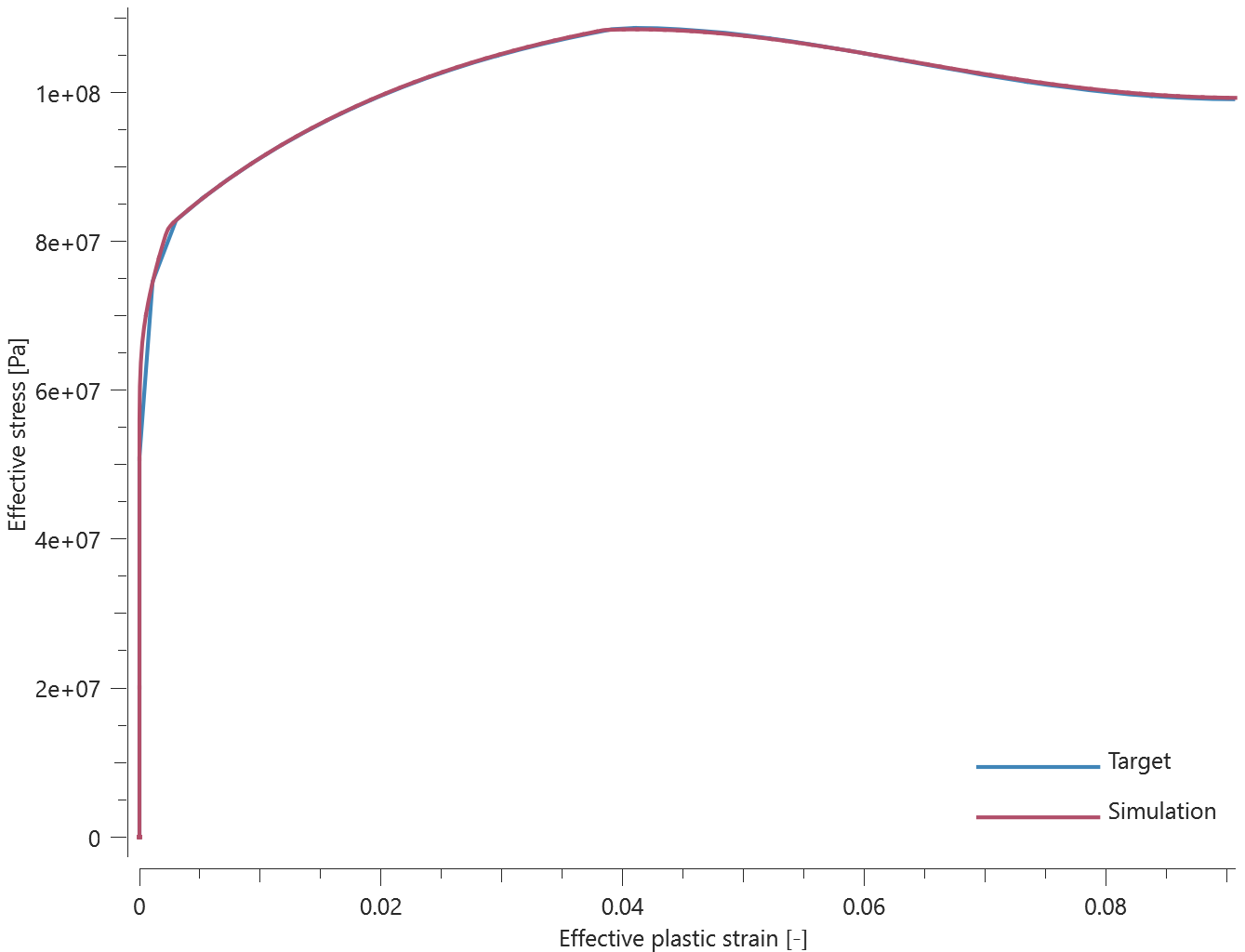
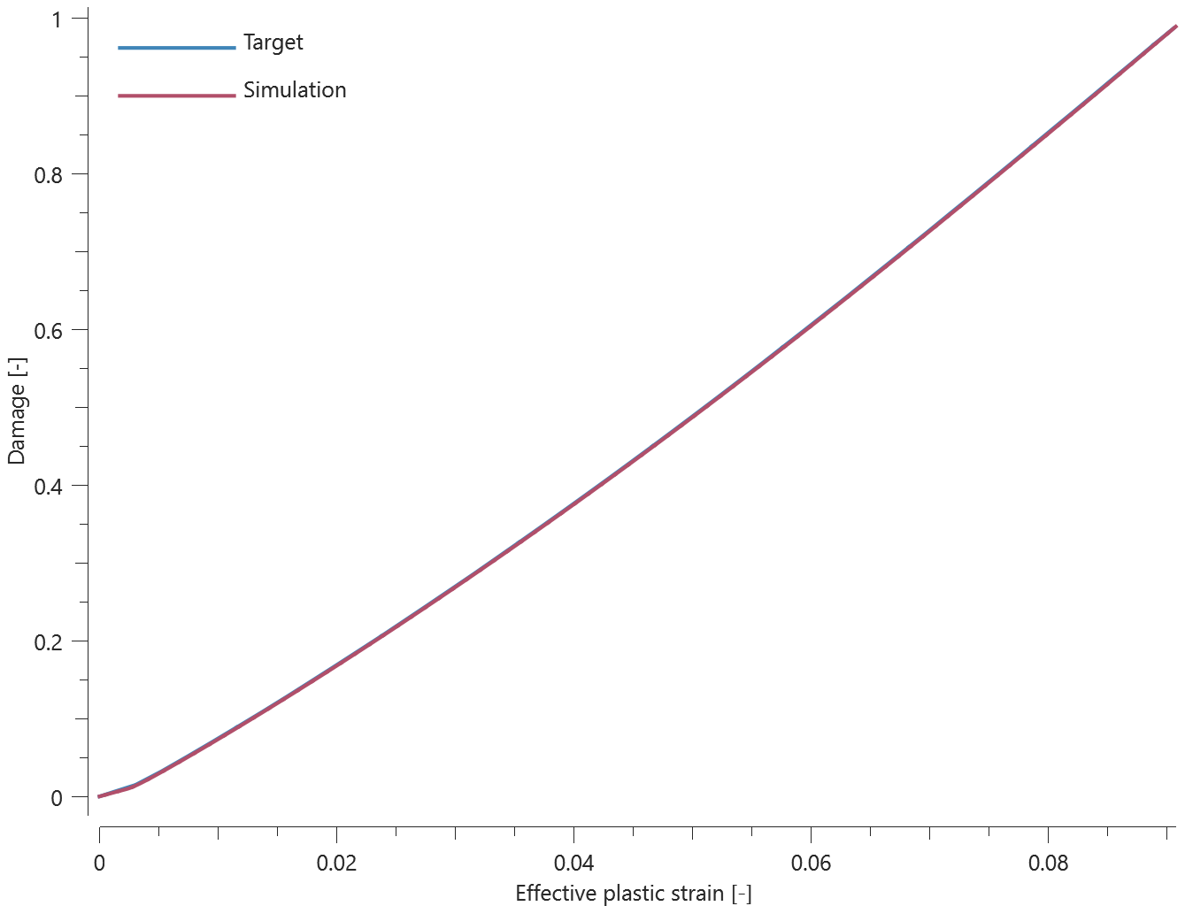
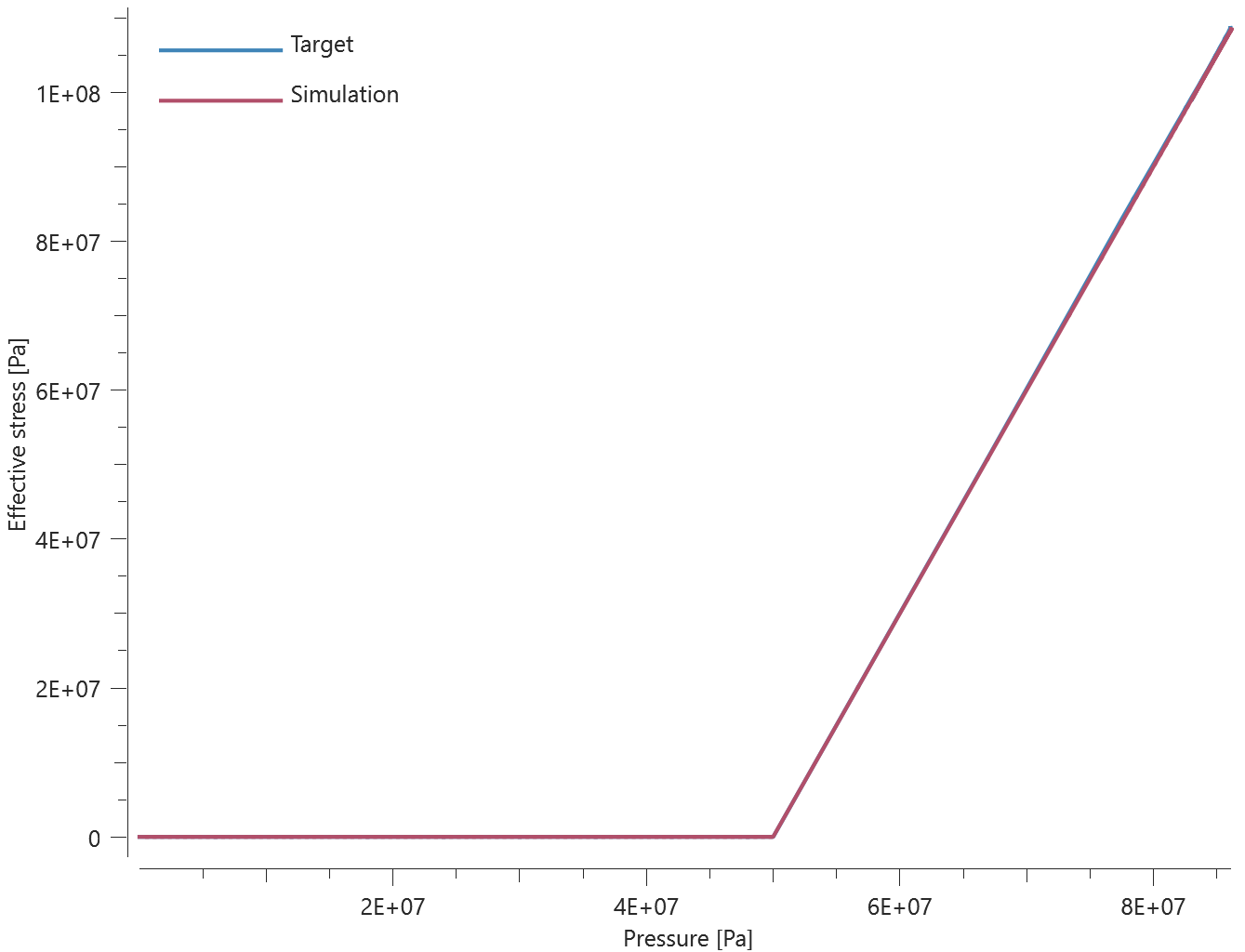
Test 11 - Dynamic, uniaxial tension
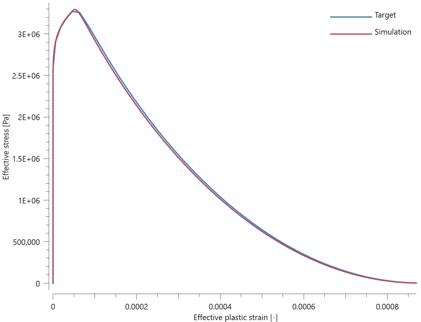
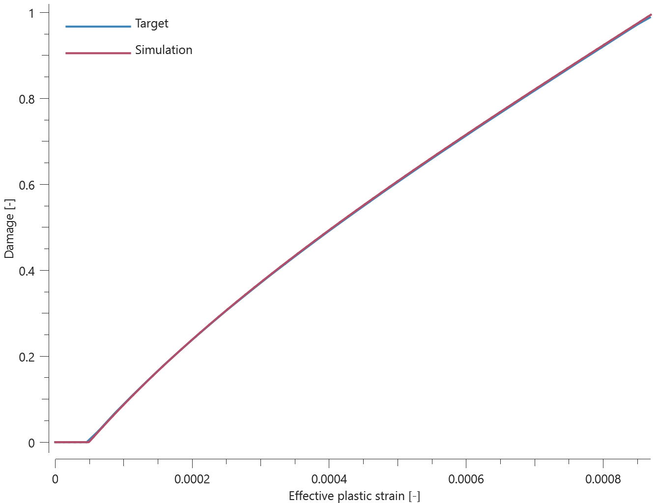
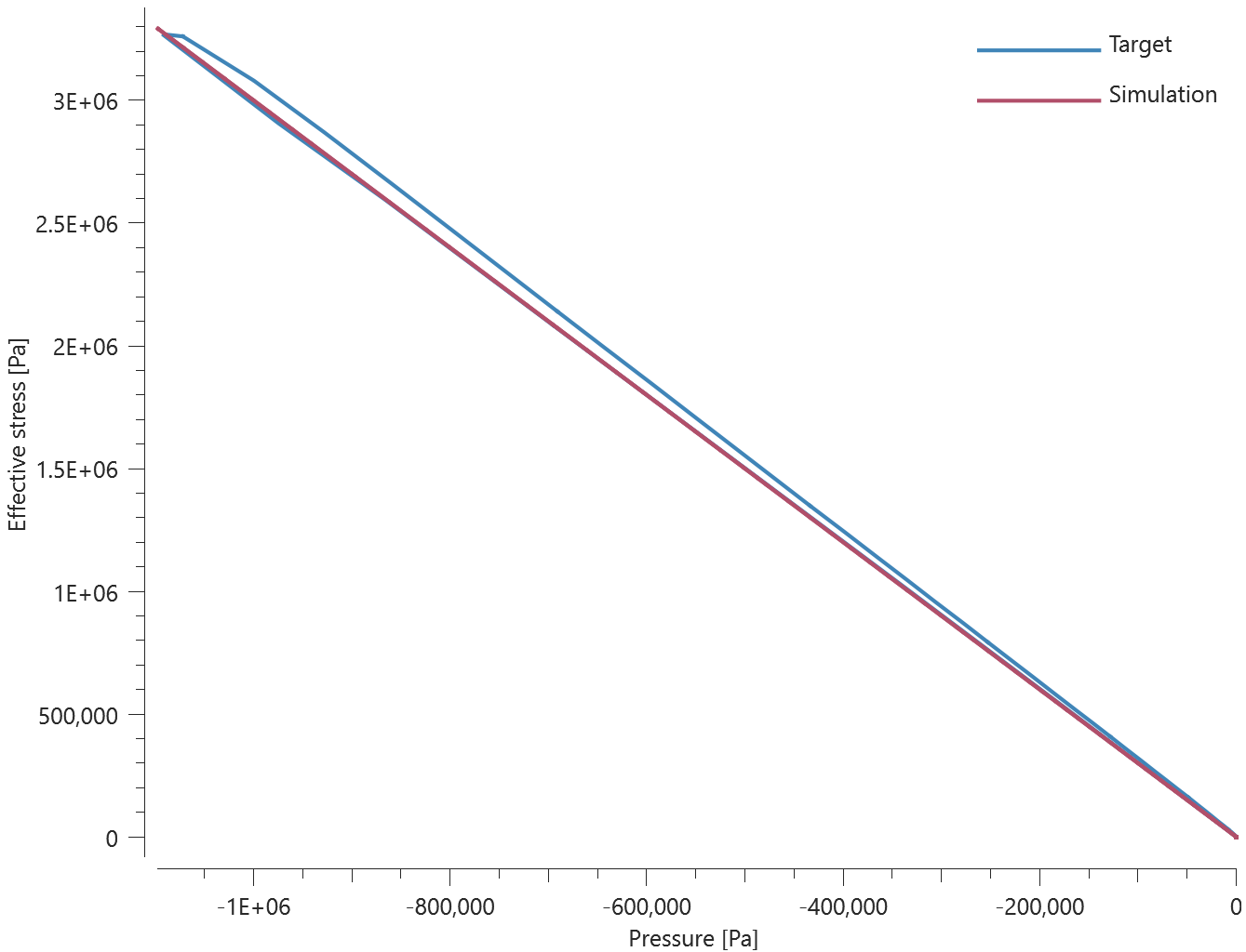
Test 12 - Dynamic, stretching at 15 MPa confinement pressure
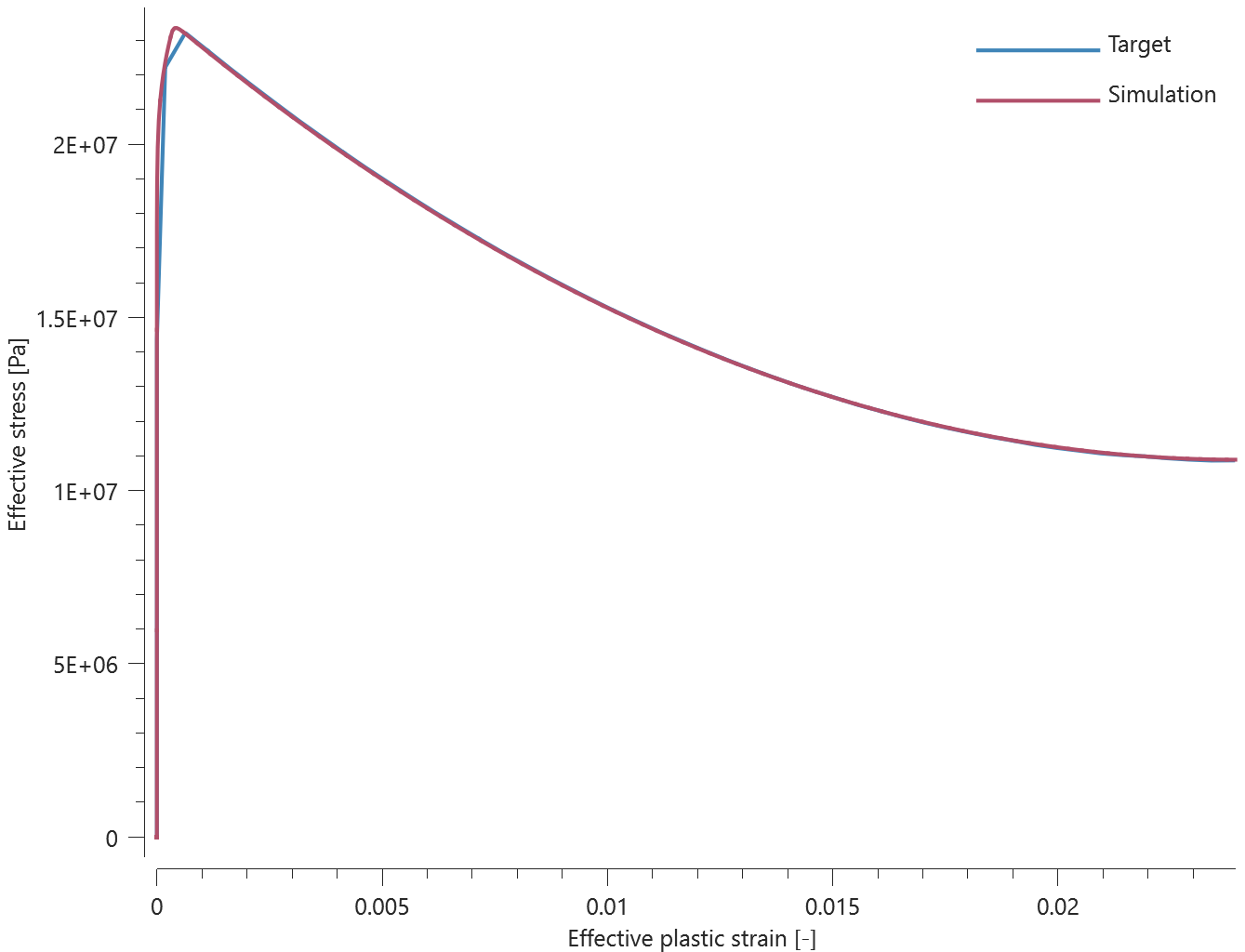
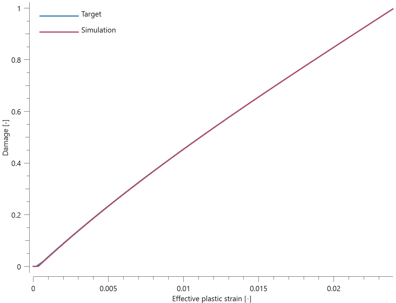
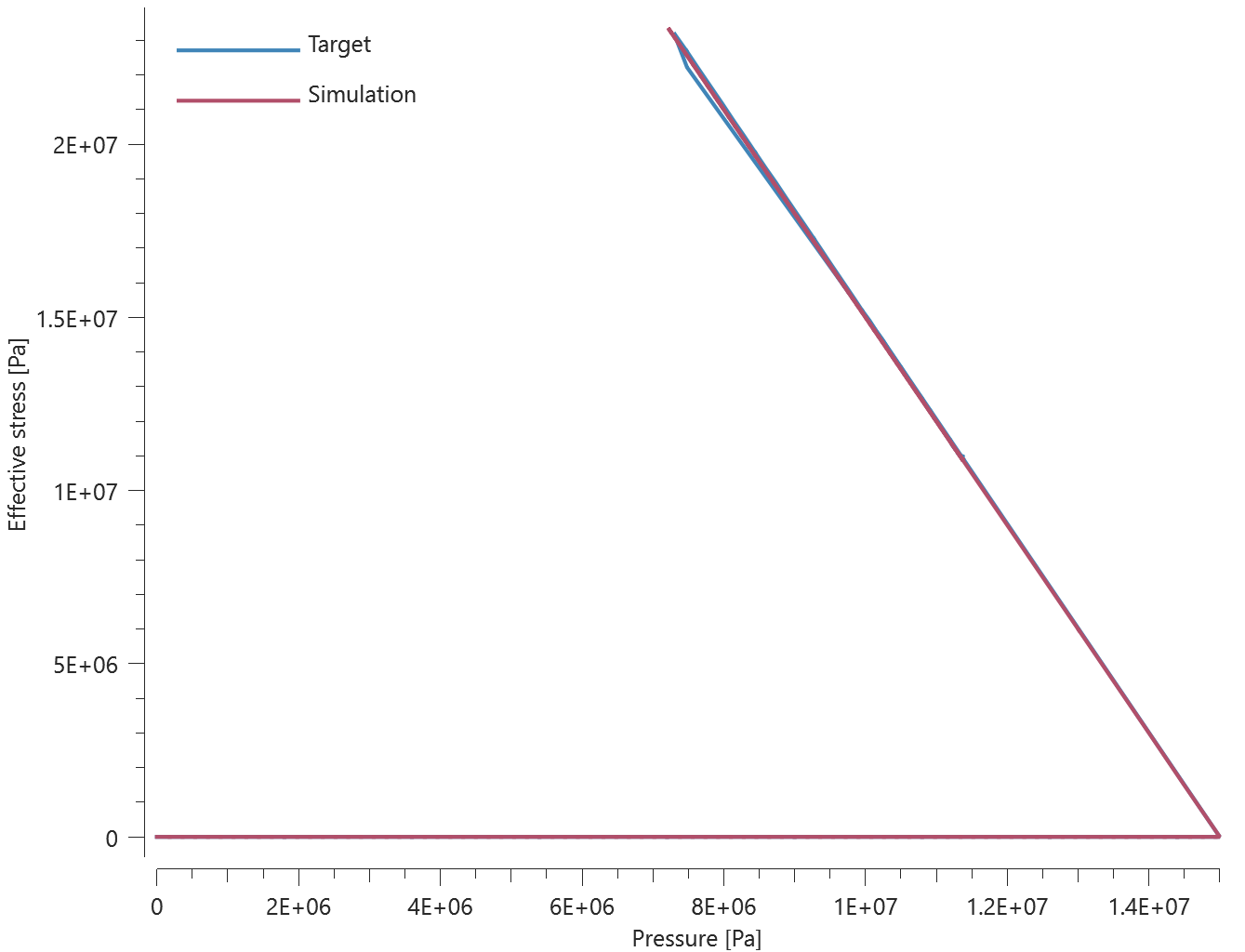
Test 13 - Dynamic, stretching at 50 MPa confinement pressure
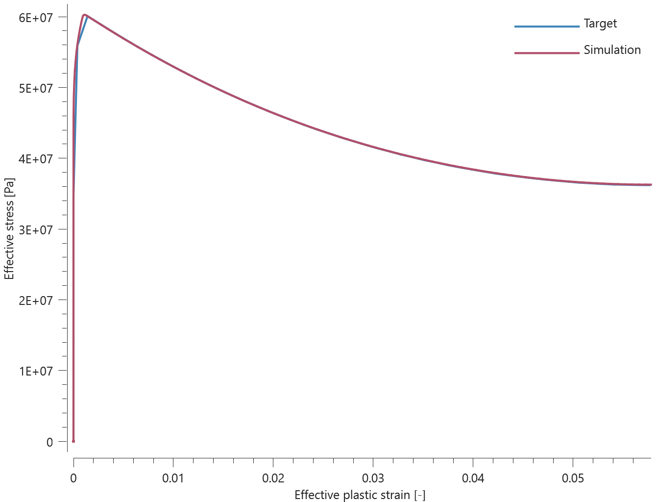
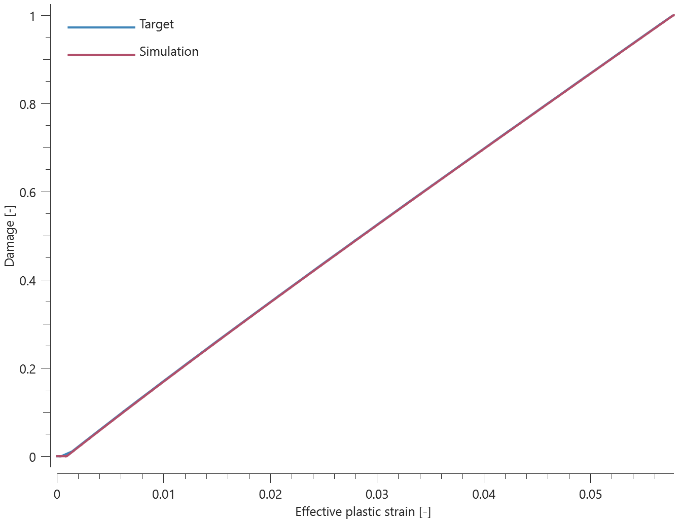
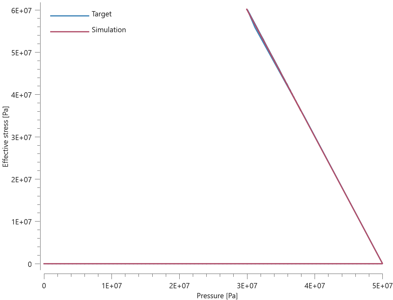
Test 14 - Dynamic, volumetric compression
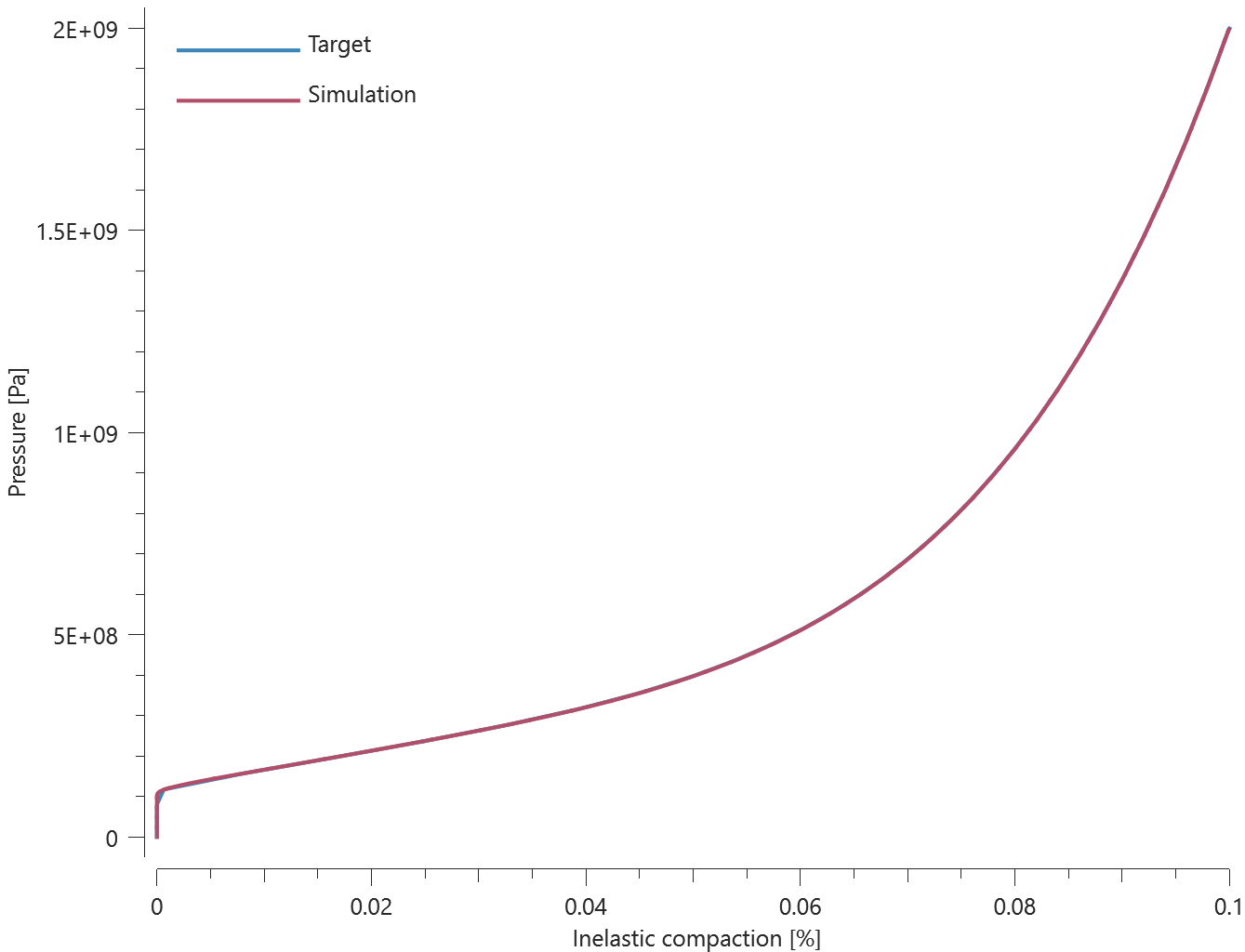
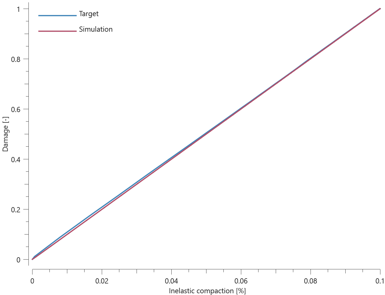

The tests presented in this document are subjected to version control.
Tests
This benchmark is associated with 14 tests.
*MAT_MM_CONCRETE_SPH
Verification_MAT_MM_CONCRETE_SPH
These tests verify that the SPH-implementation of *MAT_MM_CONCRETE operates equivalently to the FE-implementation. The test setup consists of cubes of either elements or particles. The cubes are compressed or stretched, depending on configuration. The prescribed deformation causes a state of uniaxial strain in the cubes. The models are run with and without strain rate hardening activated. Plots of effective stress vs. effective plastic strain and pressure vs. volumetric strain and are presented below. Figure 1 and 2 show the result from the cubes being compressed and Figure 3 and 4 shows results from the cubes being stretched.
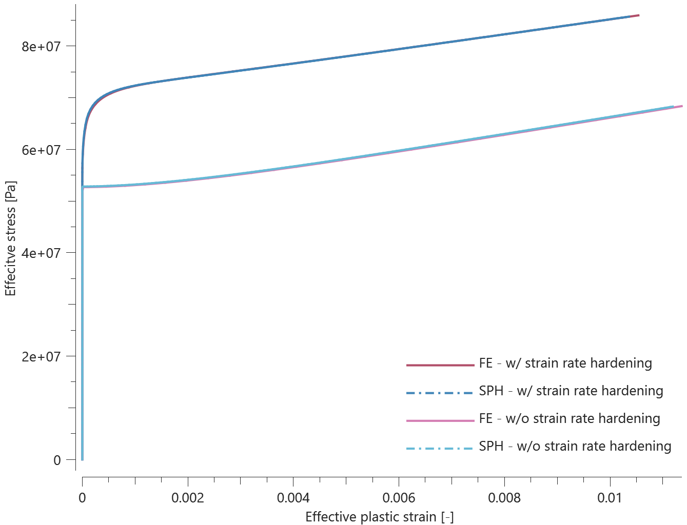
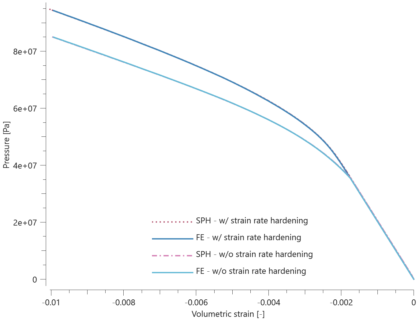
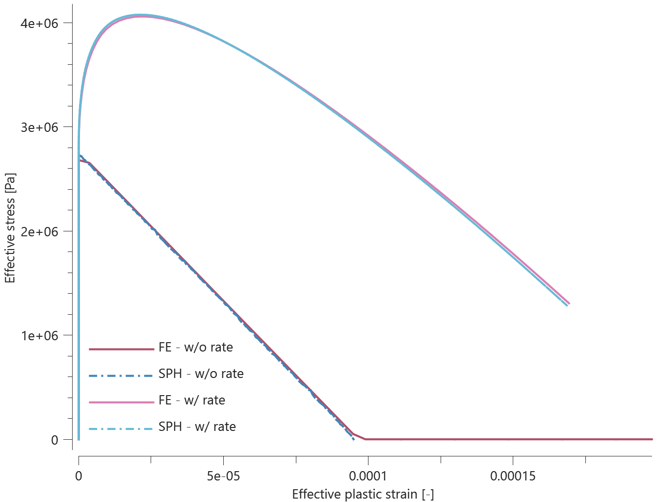
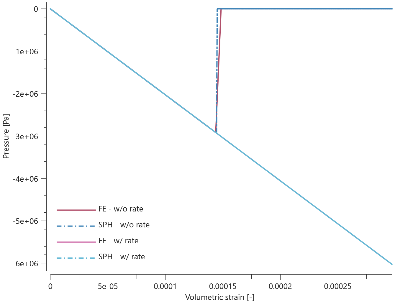
Maximum, minimum and average values of effective stress, pressure, effective plastic strain and volumetric strain are checked for version control.
Tests
This benchmark is associated with 8 tests.
*MAT_MOONEY_RIVLIN
Elasticity
"Optional title"
mid, $\rho$, $K$, ., ., tid
$C_1$, $C_2$, $\alpha_1$, $\beta_1$, $\alpha_2$, $\beta_2$, $\alpha_3$, $\beta_3$
$\alpha_4$, $\beta_4$
The elasticity in *MAT_MOONEY_RIVLIN is verified in this test.
Tested parameters: $K$, $C_1$ and $C_2$.
A CHEX element is deformed by prescribed displacements given by the following functions:
X-direction:
$$ disp \cdot (X/L) \cdot sin(360 \cdot t/ tend) $$
Y-direction:
$$0.5 \cdot disp \cdot (Y/L) \cdot sin(360 \cdot t/ tend) $$
Z-direction:
$$ -0.5 \cdot disp \cdot(Z/L) \cdot sin(360 \cdot t/ tend) $$
$disp$, $L$ and $tend$ are user-defined parameters. $disp$ is a displacement (corresponding to 40% nominal strain), $L$ is the element side length and $tend$ is the termination time.
$X$, $Y$, $Z$ and $t$ are intrinsic parameters. $X$, $Y$, $Z$ corresponds to coordinates and $t$ the current time in the simulation.
Stress in the X-, Y- and Z-direction vs. time and pressure vs. time from the element are presented in Figure 1 and 2 together with target curves obtained from a verification script.
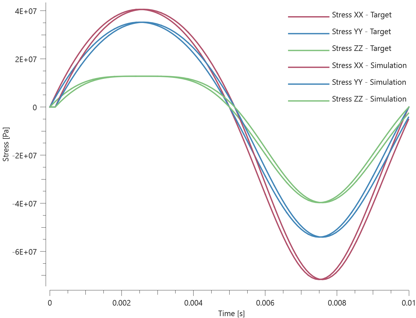

Maximum and average value of stress in the X-, Y- and Z-direction and pressure are checked.
Tests
This benchmark is associated with 1 tests.
Visco-elasticity
"Optional title"
mid, $\rho$, $K$, ., ., tid
$C_1$, $C_2$, $\alpha_1$, $\beta_1$, $\alpha_2$, $\beta_2$, $\alpha_3$, $\beta_3$
$\alpha_4$, $\beta_4$
The viscosity in *MAT_MOONEY_RIVLIN is verified in this test.
Tested parameters: $\alpha_1$ - $\alpha_4$ and $\beta_1$ - $\beta_4$.
A CHEX element is deformed by prescribed displacements given by the following functions:
X-direction:
$$ disp \cdot (X/L) \cdot sin(360 \cdot t/ tend) $$
Y-direction:
$$ 0.5 \cdot disp \cdot (Y/L) \cdot sin(360 \cdot t/ tend) $$
Z-direction:
$$ -0.5 \cdot disp \cdot(Z/L) \cdot sin(360 \cdot t/ tend) $$
$disp$, $L$ and $tend$ are user-defined parameters. $disp$ is a displacement (corresponding to 40% nominal strain), $L$ is the element side length and $tend$ is the termination time.
$X$, $Y$, $Z$ and $t$ are intrinsic parameters. $X$, $Y$, $Z$ corresponds to coordinates and $t$ the current time in the simulation.
Stress in the X-, Y- and Z-direction vs. time and pressure vs. time from the element are presented in Figure 1 and 2 together with target curves obtained from a verification script.
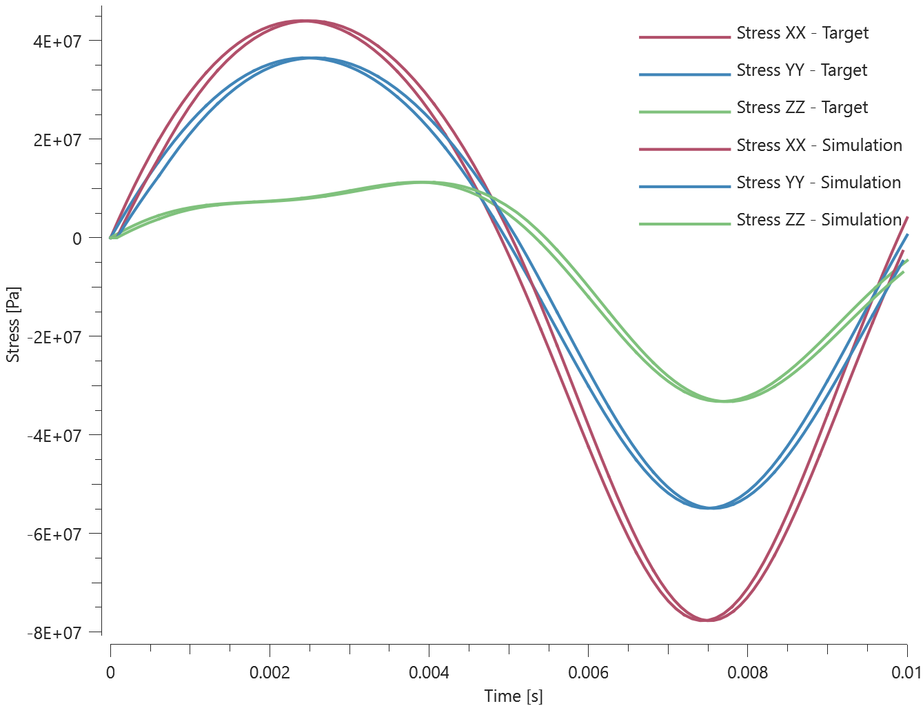
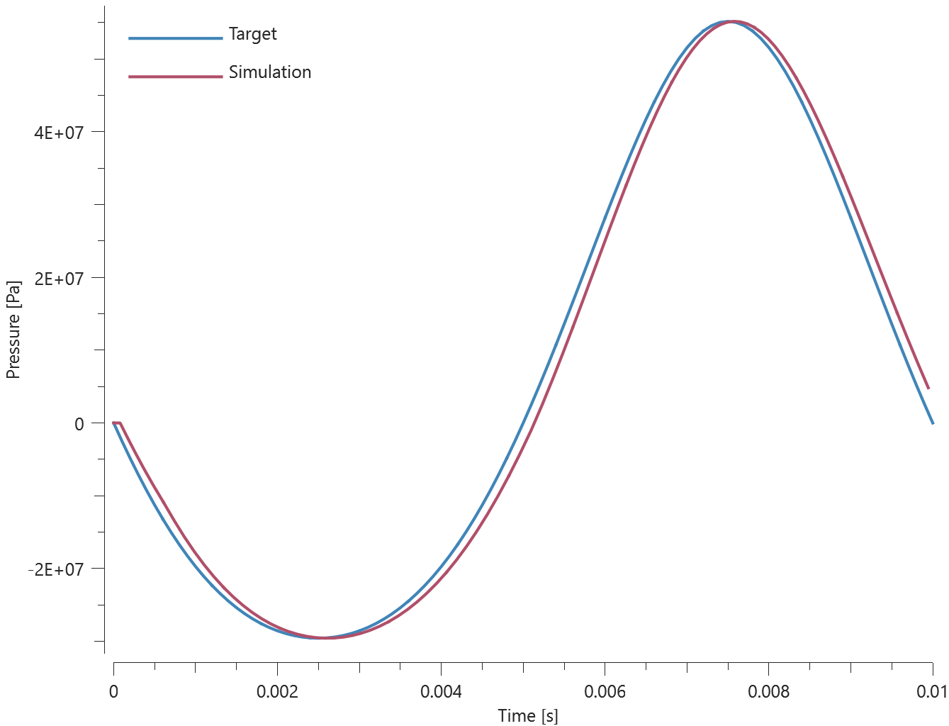
Maximum and average value of stress in the X-, Y- and Z-direction and pressure are checked.
Tests
This benchmark is associated with 1 tests.
*MAT_MULTILAYER_ORTHOTROPIC
Elasticity (Youngs moduli and Poissons ratios)
"Optional title"
mid, $\rho$, $E_1$, $E_2$, $G_{12}$, $\nu_{12}$
$E_3$, $G_{13}$, $G_{23}$, $\nu_{13}$, $\nu_{23}$, $\varepsilon_t$, $\varepsilon_c$, erode
ndir, $\alpha_1$, ..., $\alpha_7$
$c$
The Young's moduli and Poisson's ratios in *MAT_MULTILAYER_ORTHOTROPIC are verified in this test.
Tested parameters: $E_1$, $E_2$, $E_3$, $\nu_{12}$, $\nu_{23}$ and $\nu_{31}$.
Three CHEX elements are stretched in the global X-direction while fixed in the Y- and Z-direction. The local x- and y-directions in each element, expressed in global directions, are presented in Table 1.
| Test | Local x-axis, [X, Y, Z] | Local y-axis, [X, Y, Z] | Tested parameters |
|---|---|---|---|
| 1 | [1, 0, 0] | [0, 1, 0] | $E_1$, $\nu_{12}$, $\nu_{13}$ |
| 2 | [0, 0, 1] | [1, 0, 0] | $E_2$, $\nu_{12}$, $\nu_{23}$ |
| 3 | [0, 1, 0] | [0, 0, 1] | $E_3$, $\nu_{13}$, $\nu_{23}$ |
Stress in X-, Y- and Z- direction for each element is presented in Figure 1- 3 together with target curves from a verification script.
/mat_multilayer_orthotropic_elasticity_youngs_modulus_element_1.png)
/mat_multilayer_orthotropic_elasticity_youngs_modulus_element_2.png)
/mat_multilayer_orthotropic_elasticity_youngs_modulus_element_3.png)
Maximum and average stress in X-, Y- and Z-direction are checked in the elements.
Tests
This benchmark is associated with 1 tests.
Elasticity (shear moduli)
"Optional title"
mid, $\rho$, $E_1$, $E_2$, $G_{12}$, $\nu_{12}$
$E_3$, $G_{13}$, $G_{23}$, $\nu_{13}$, $\nu_{23}$, $\varepsilon_t$, $\varepsilon_c$, erode
ndir, $\alpha_1$, ..., $\alpha_7$
$c$
The shear moduli in *MAT_MULTILAYER_ORTHOTROPIC are verified in this test.
Tested parameters: $G_{12}$, $G_{23}$ and $G_{13}$.
Three CHEX elements are sheared in the global XY-direction. The local x- and y-direction in each element, expressed in global directions, are presented in Table 1.
| Test | Local x-axis, [X, Y, Z] | Local y-axis, [X, Y, Z] | Tested parameters |
|---|---|---|---|
| 1 | [1, 0, 0] | [0, 1, 0] | $G_{12}$ |
| 2 | [0, 0, 1] | [1, 0, 0] | $G_{23}$ |
| 3 | [0, 1, 0] | [0, 0, 1] | $G_{13}$ |
Stress XY (global) vs. time from the elements are presented in Figure 1 together with target curves from a verification script.
/mat_multilayer_orthotropic_elasticity_shear_moduli.png)
Maximum and average stress are checked in the elements.
Tests
This benchmark is associated with 1 tests.
Fiber failure criteria
"Optional title"
mid, $\rho$, $E_1$, $E_2$, $G_{12}$, $\nu_{12}$
$E_3$, $G_{13}$, $G_{23}$, $\nu_{13}$, $\nu_{23}$, $\varepsilon_t$, $\varepsilon_c$, erode
ndir, $\alpha_1$, ..., $\alpha_7$
$c$
The fiber fracture criteria in *MAT_MULTILAYER_ORTHOTROPIC are verified in this test.
Tested parameters: $\varepsilon_t$, $\varepsilon_c$, ndir and $\alpha_1$.
Six CHEX elements are used in this test. Loading conditions, loading directions and fiber orientations for the elements are presented in Table 1.
| Element ID | Loading condition | Loading direction | Fiber orientation |
|---|---|---|---|
| 1 | tension | X | X |
| 2 | Compression | X | X |
| 3 | tension | X | Y |
| 4 | Compression | X | Y |
| 5 | tension | X | Z |
| 6 | Compression | X | Z |
Both $\varepsilon_t$ and $\varepsilon_c$ assumes non-zero values. The strain at termination exceeds the failure strain. Fiber failure only occurs in element 1 and 2 since the loading direction coincides with the fiber direction in these elements. Effective stress vs. time from the elements is presented in Figure 1 - 3.
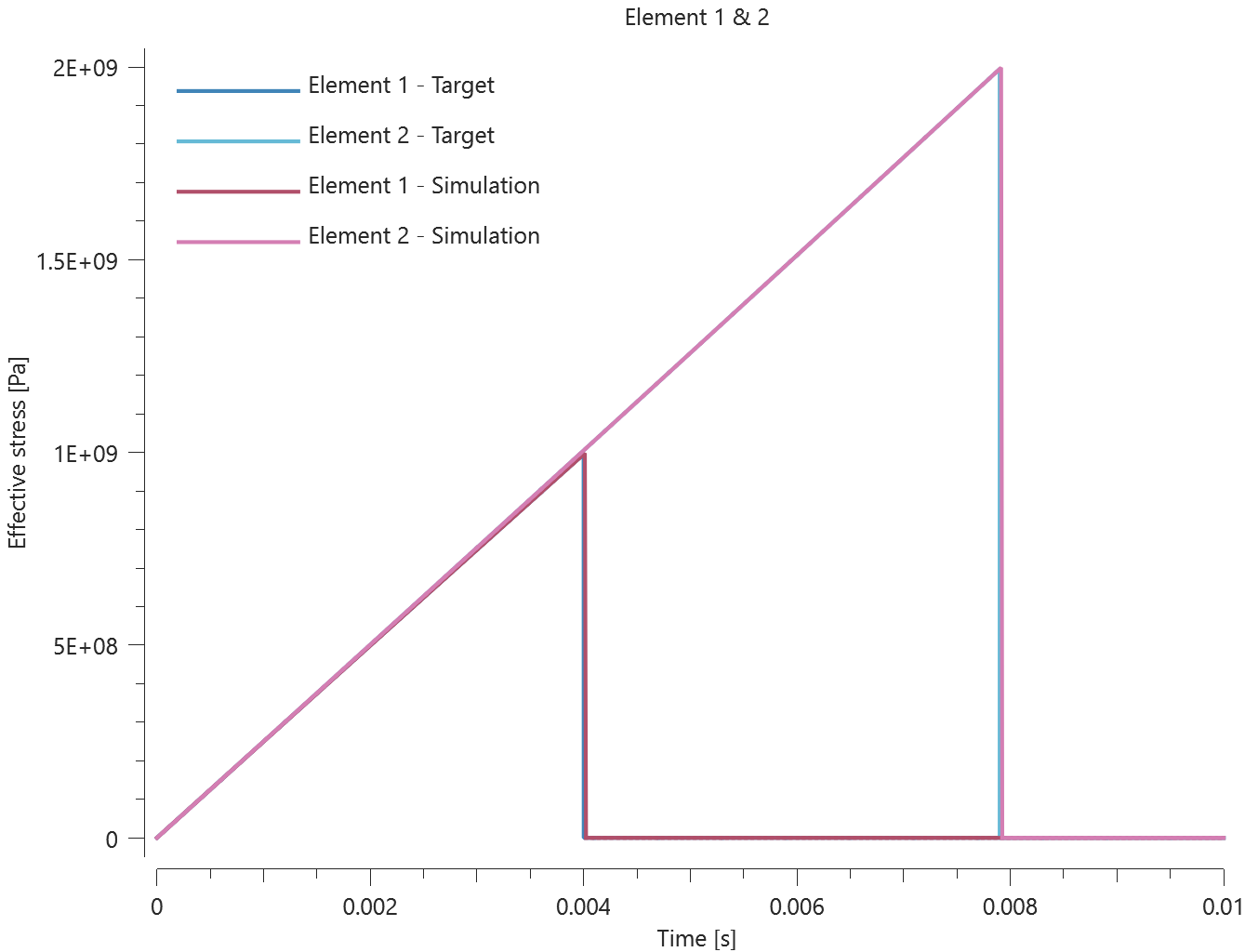
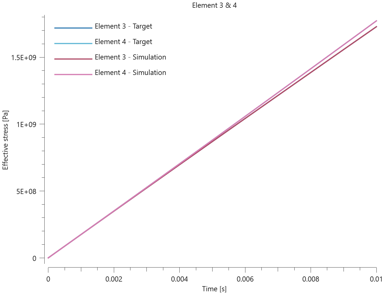
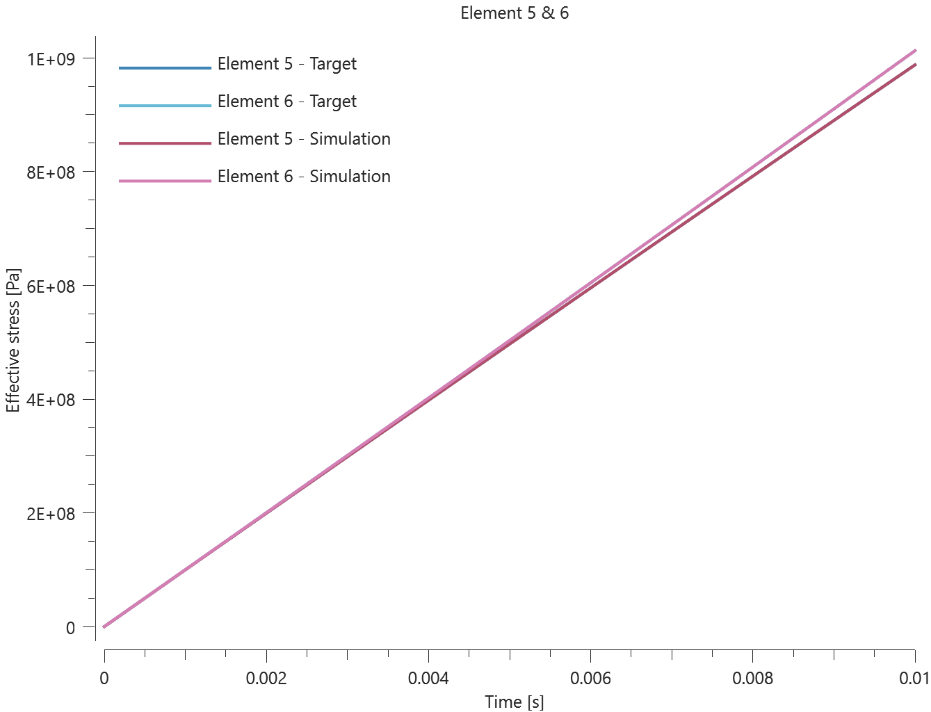
Maximum and average effective stress are checked in the elements.
Tests
This benchmark is associated with 1 tests.
Strain rate effects
"Optional title"
mid, $\rho$, $E_1$, $E_2$, $G_{12}$, $\nu_{12}$
$E_3$, $G_{13}$, $G_{23}$, $\nu_{13}$, $\nu_{23}$, $\varepsilon_t$, $\varepsilon_c$, erode
ndir, $\alpha_1$, ..., $\alpha_7$
$c$
The strain rate effect in *MAT_MULTILAYER_ORTHOTROPIC is verified in this test.
Tested parameters: $c$.
A CHEX element is stretched in the X-direction while fixed in the Y- and Z-direction. The deformation is caused by a prescribed strain rate. Stress in X-, Y- and Z-direction vs. time is presented in Figure 1 together with target curves from a verfication script.
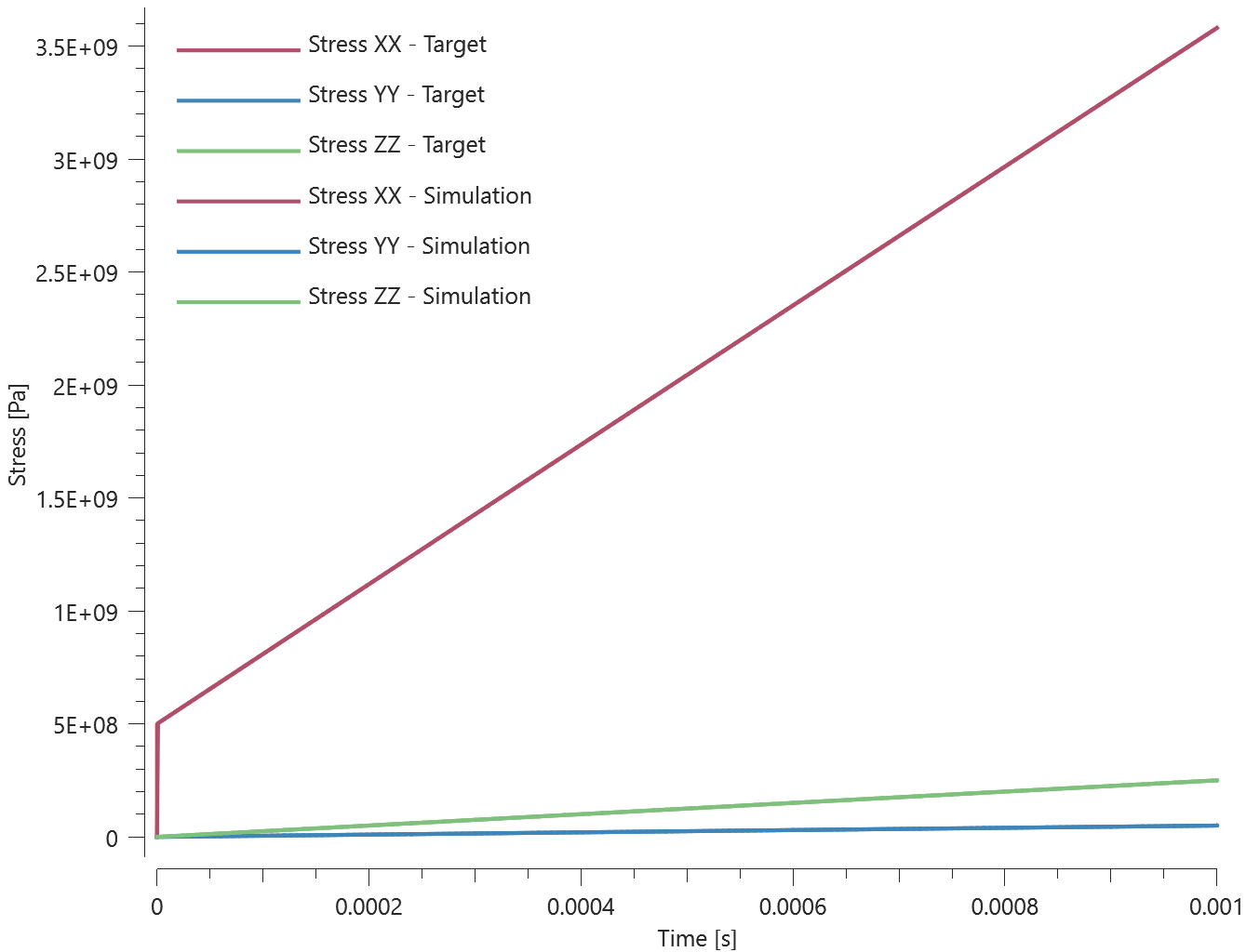
Maxmimum and average stress in the X-, Y- and Z-direction are checked.
Tests
This benchmark is associated with 1 tests.
*MAT_ORTHOTROPIC
Elasticity (Youngs moduli and Poissons ratio)
"Optional title"
mid, $\rho$, $E_1$, $E_2$, $G_{12}$, $\nu_{12}$, $\nu_{23}$
$c$, $c_{dec}$, $X_t$, $X_c$, $Y_t$, $Y_c$, $\beta$, $S$
erode, $res$
The Young's moduli and Poisson's ratios in *MAT_ORTHOTROPIC are verified in this test.
Tested parameters: $E_1$, $E_2$, $\nu_{12}$ and $\nu_{23}$.
A CHEX with fibers defined in the X-direction is used in this test. The element is stretched in the fiber direction while fixed in the other directions. Stress in X-, Y- and Z-direction vs. time are presented in Figure 1 together with target curves from a verification script.
/mat_orthotropic_elasticity_youngs_modulus.png)
Maximum and average stress in X-, Y- and Z-direction are checked.
Tests
This benchmark is associated with 1 tests.
Elasticity (shear modulus)
"Optional title"
mid, $\rho$, $E_1$, $E_2$, $G_{12}$, $\nu_{12}$, $\nu_{23}$
$c$, $c_{dec}$, $X_t$, $X_c$, $Y_t$, $Y_c$, $\beta$, $S$
erode, $res$
The shear modulus in *MAT_ORTHOTROPIC is verified in this test.
Tested parameters: $G_{12}$.
Two CHEX elements are sheared in the XY-direction. In one of the elements, the fiber direction is defined in the X-direction and in the other in the Z-direction. The stress in XY-direction vs. time in both elements are presented in Figure 1 together with target curves from a verifcation script.
/mat_orthotropic_elasticity_shear_modulus.png)
Maximum and average stress in XY are checked in the elements.
Tests
This benchmark is associated with 1 tests.
Fiber failure criteria
"Optional title"
mid, $\rho$, $E_1$, $E_2$, $G_{12}$, $\nu_{12}$, $\nu_{23}$
$c$, $c_{dec}$, $X_t$, $X_c$, $Y_t$, $Y_c$, $\beta$, $S$
erode, $res$
The fiber failure criteria in *MAT_ORTHOTROPIC are verified in this test.
Tested parameters: $X_t$, $X_c$ and $res$.
Two CHEX elements are used in this test. One element is stretched and the other compressed. The elements are fixed in the directions perpendicular to the stretching/compression.
Stress in the fiber direction vs. time from the elements are presented in Figure 1 and 2 together with target curves from a verification script.
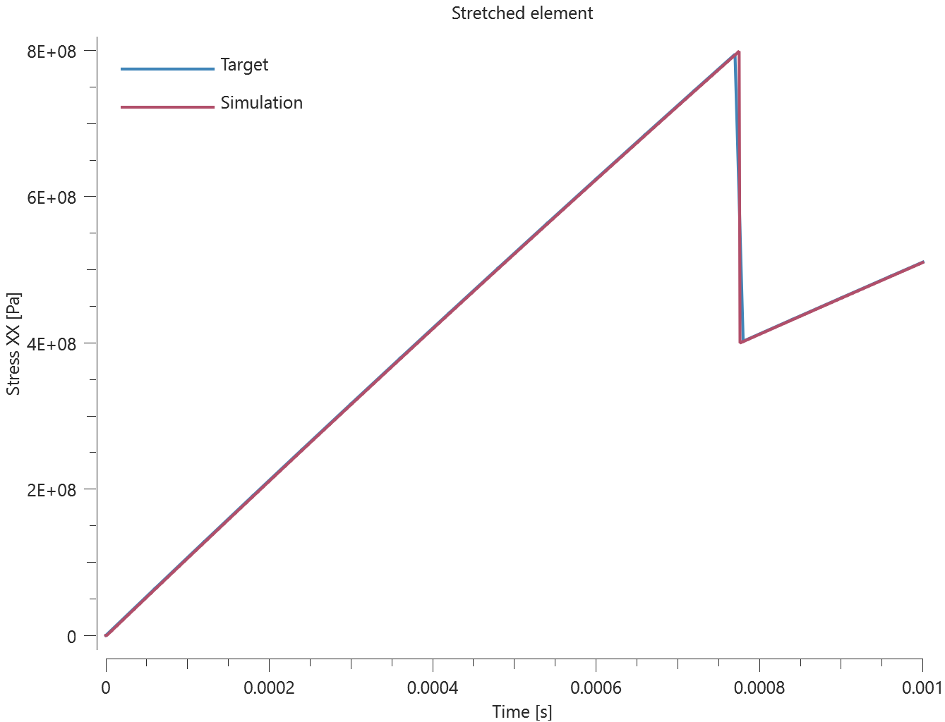
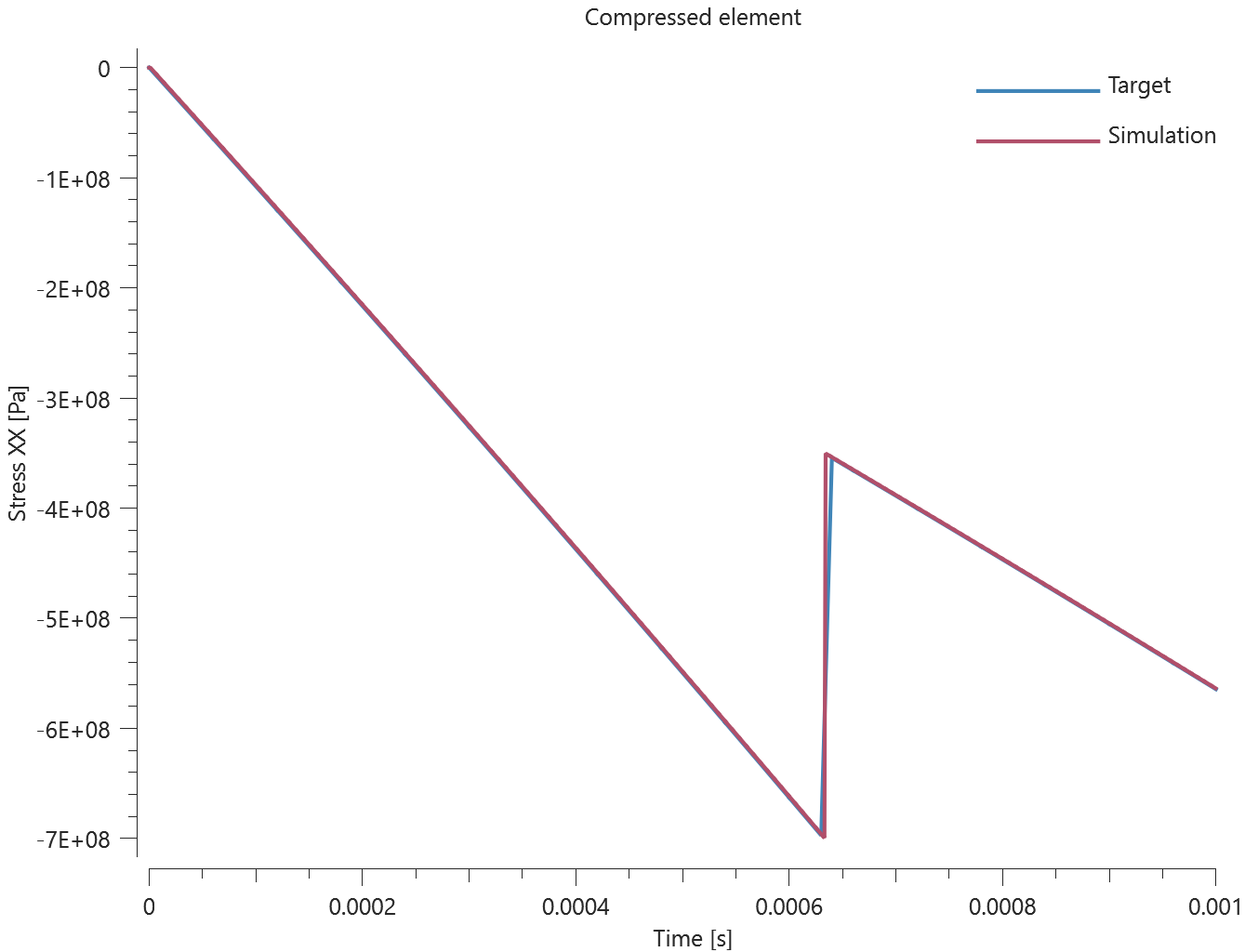
Maximum, minimum and average stress in the fiber direction are checked in the elements.
Tests
This benchmark is associated with 1 tests.
Viscous damping
"Optional title"
mid, $\rho$, $E_1$, $E_2$, $G_{12}$, $\nu_{12}$, $\nu_{23}$
$c$, $c_{dec}$, $X_t$, $X_c$, $Y_t$, $Y_c$, $\beta$, $S$
erode, $res$
The viscous damping in *MAT_ORTHOTROPIC is verified in this test.
Tested parameters: $c$ and $c_{dec}$.
Two CHEX elements are stretched in the X-direction while fixed in the Y- and Z-direction. Damping is active in one the elements. Stress in the X-direction vs. time from both elements is presented in Figure 1 together with target curves from a verification script.
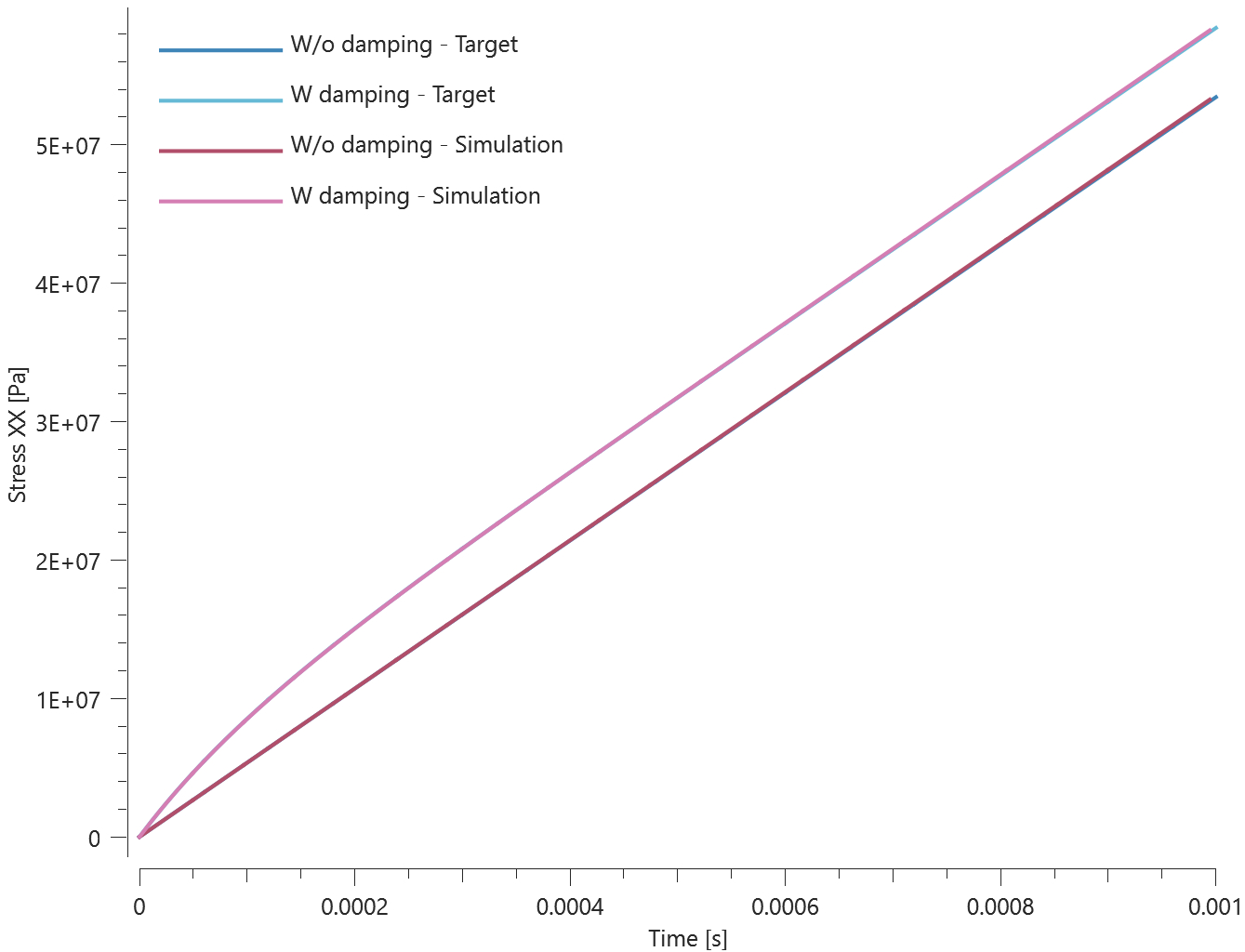
Maximum and average stress are checked in both elements.
Tests
This benchmark is associated with 1 tests.
*MAT_POWDER_BURN
Interior ballistics
"Optional title"
mid, $\rho$, $E$, $\nu$, did
$C_v$, $\gamma$, $e_0$, $v$, fid, $T_i$, $p_i$
local, $A$, $B$, $n$
Tested parameters: mid, $\rho$, $C_v$, $\gamma$, $e_0$, $v$, fid, $T_i$, $p_i$.
This model tests propellant grains burning in a simple internal ballistics demonstration model. The model consists of a projectile inside a barrel and propellant with material properties defined with *MAT_POWDER_BURN. The command is used to model unburned propellant as rigid or elasto-plastic grains and its combustion products as discrete particles. See Figure 1.
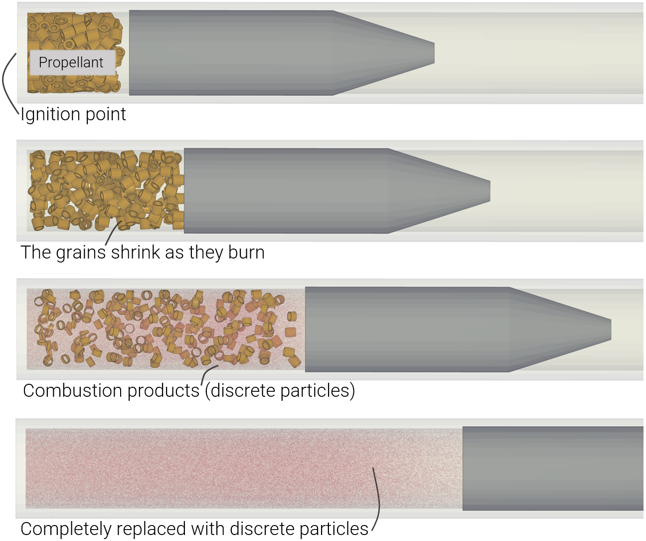
The specific test assumptions are:
- Grains assumed rigid and a particle domain is defined for the combustion products.
- An ignition point is assigned with *POWDER_BURN_IGNITE.
- The projectile is given restricted motion in all directions except Z-direction.
- Contact is defined between the propellant to the barrel and projectile.
- Particle-structure contact is defined in the particle domain.
Propellant grains replaced by combustion products can be seen in Figure 2.

Velocity of the projectile can be seen in Figure 3.
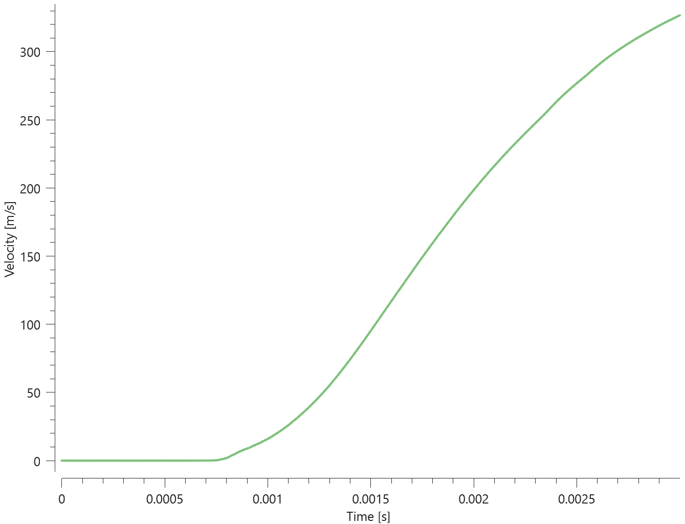
The burn rate of the propellant is checked in slowburn.out. Also, velocity of the projectile and the combustion products (number of particles) is checked for version control.
Tests
This benchmark is associated with 1 tests.
*MAT_POWDER_BURN_POURUS
Gas pressure
"Optional title"
mid, $\rho$, $E$, $\nu$
$C_v$, $\gamma$, $e_0$, $b$, fid, $T_i$, $p_i$, $t_i$
$\eta_0$, $A$, $B$, $n$
This tests the *MAT_POWDER_BURN_POURUS command. A cylinder of powder is placed on a rigid plate in a CFD domain. Once the simulation starts the powder will react with the surrounding gas and ignite. The pressure in the CFD domain is then compared to an analytically calculated pressure according to:
$$ p = \frac{\gamma - 1}{1 - \rho_{CFD}b} e $$
Model at initiation can be seen in Figure 1.
The simulated pressure together with the analytical caluculated target can be found in Figure 2.
The last value of pressure in the CFD domain is checked.
Tests
This benchmark is associated with 1 tests.
*MAT_REBAR
Bending stiffness
"Optional title"
mid, $\rho$, $E$
cid, $c$, $\dot{\varepsilon}_0$, $W_c$, $\tau_{max}$, bend, $r_{ref}$
The optional bending stiffness in *MAT_REBAR is verified in this test.
Tested parameter: bend.
Two simply supported beams are subjected to a mid-span displacement, $\Delta$. The height and width of the quadratic cross section is $w$, the length is $L$ ($L >> w$) and Young's modulus is $Eb$.
The beams are reinforced with a rebar with diameter $d$, length $L$ and Young's modulus $Er$. The rebar is positioned in the center of beams cross section.
Bending stiffness is active in one of the beams.
Maximum reaction force in the beam without bending stiffness in rebar:
$$ P_0 = \frac{48 \cdot Eb \cdot Ib \cdot \Delta}{L^3} $$
where $Ib = w^4/12$.
Maximum reaction force in the beam with bending stiffness in rebar:
$$ P_1 = \frac{48 \left( Eb \cdot Ib + \cdot Er \cdot Ir \right) \cdot \Delta}{L^3} $$
where $Ir = pi \cdot (d/2)^4/4$.
The reaction forces vs. time in the beams are presented in Figure 1 together with the targets based on the calculations above.
Maximum and average reaction forces are checked in both beams.
Tests
This benchmark is associated with 1 tests.
Concrete-rebar interface shear resistance as a function of tangential slip
"Optional title"
mid, $\rho$, $E$
cid, $c$, $\dot{\varepsilon}_0$, $W_c$, $\tau_{max}$, bend, $r_{ref}$
Concrete-rebar interface shear resistance as a function of tangential slip is verified in this test.
Tested parameters: $\tau_{max}$.
A rebar element is partly embedded in a concrete cylinder. The lateral surface of the cylinder is fixed in the X-direction. A prescribed motion is imposed on the rebar end that is not embedded, pulling the rebar out of the cylinder. An image of the model is presented in Figure 1.

The interface shear resistance is defined as a function of tangential slip.
Shear stress vs. tangential slip is extracted from a sensor located in the rebar. The extracted curve is compared to the curve of shear resistance vs. tangential slip used as input. The two curves are presented in Figure 2

Maximum and average shear stress are checked for version control.
Tests
This benchmark is associated with 1 tests.
Damage
"Optional title"
mid, $\rho$, $E$
cid, $c$, $\dot{\varepsilon}_0$, $W_c$, $\tau_{max}$, bend, $r_{ref}$
Damage in *MAT_REBAR is verfied in this test.
Tested parameter: $W_c$.
The ends of a rebar are embedded in solid elements and a motion is imposed on the solid elements, causing tension in the rebar. Axial stress vs. time and damage vs. plastic strain from a sensor located in the center of the rebar element are presented in Figure 1 and 2 together with target curves from a verification script.
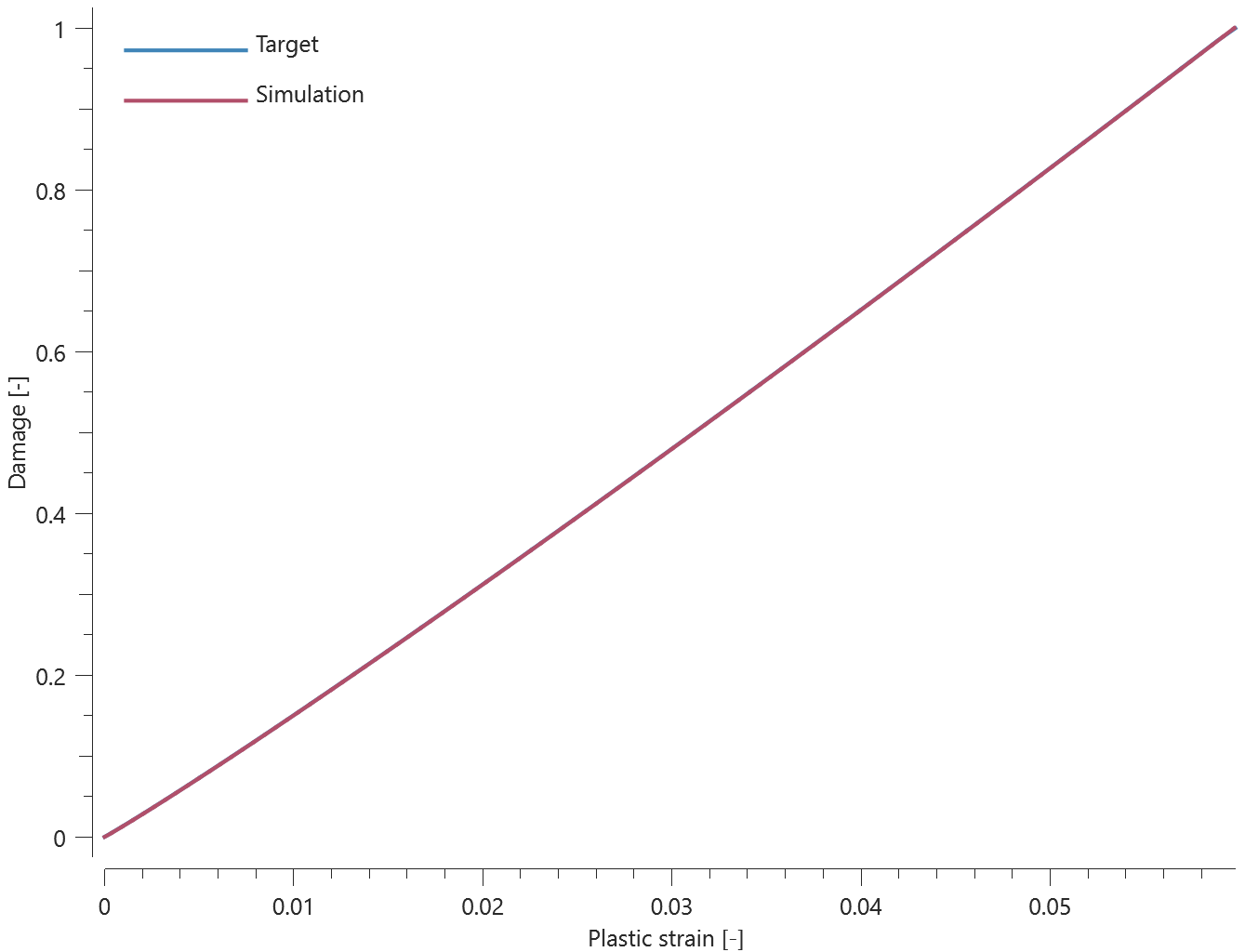
Maximum and average axial stress and damage are checked.
Tests
This benchmark is associated with 1 tests.
Max shear stress
"Optional title"
mid, $\rho$, $E$
cid, $c$, $\dot{\varepsilon}_0$, $W_c$, $\tau_{max}$, bend, $r_{ref}$
The optional interface failure in *MAT_REBAR is verfied in this test.
Tested parameters: $\tau_{max}$.
The ends of a rebar are embedded in solid elements and a motion is imposed on the solid elements, causing tension in the rebar. The diameter of the rebar is $d$, and the length of the rebar-solid element interface is $\Delta$.
The maximum axial stress, $\sigma_{max}$, in the rebar prior to interface failure is calculated as:
$$ \sigma_{max} = F_a / A_a $$
$F_a$ is the normal force in the rebar and $A_a$ is the cross-sectional area:
$$ A_a = \pi \cdot d^2/4 $$
$F_a$, is equal to the shear force, $F_s$, which is calculated as:
$$ F_s = \tau_{max} \cdot A_s $$
$A_s$ is the area of the interface:
$$ A_s = \pi \cdot d \cdot \Delta $$
The maximum axial stress can be expressed as:
$$ \sigma_{max} = \tau_{max} \cdot A_s / A_a = 4 \cdot \tau_{max} \cdot \Delta/d $$
The axial stress vs. time from the rebar element is presented in Figure 1 together with the target based on the calculations above.
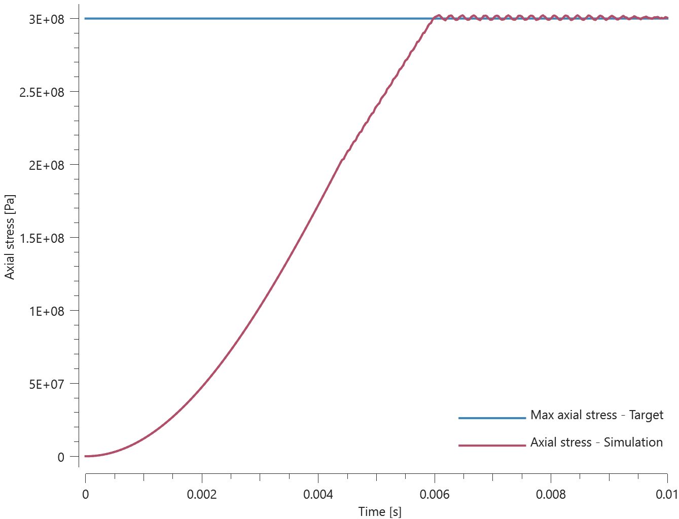
Maximum and average axial stress are checked.
Tests
This benchmark is associated with 1 tests.
Strain rate effect
"Optional title"
mid, $\rho$, $E$
cid, $c$, $\dot{\varepsilon}_0$, $W_c$, $\tau_{max}$, bend, $r_{ref}$
The dynamic yield stress in *MAT_REBAR is verfied in this test.
Tested parameters: $E$, cid, $c$, $\dot{\varepsilon}_0$.
The ends of a rebar are embedded in solid elements and a motion is imposed on the solid elements, causing tension in the rebar. The strain rate parameters are selected to have a significant effect on the yield stress.
Axial stress vs. plastic strain from a sensor located in the center of the rebar element is presented in Figure 1 together with a target curve from a verification script.
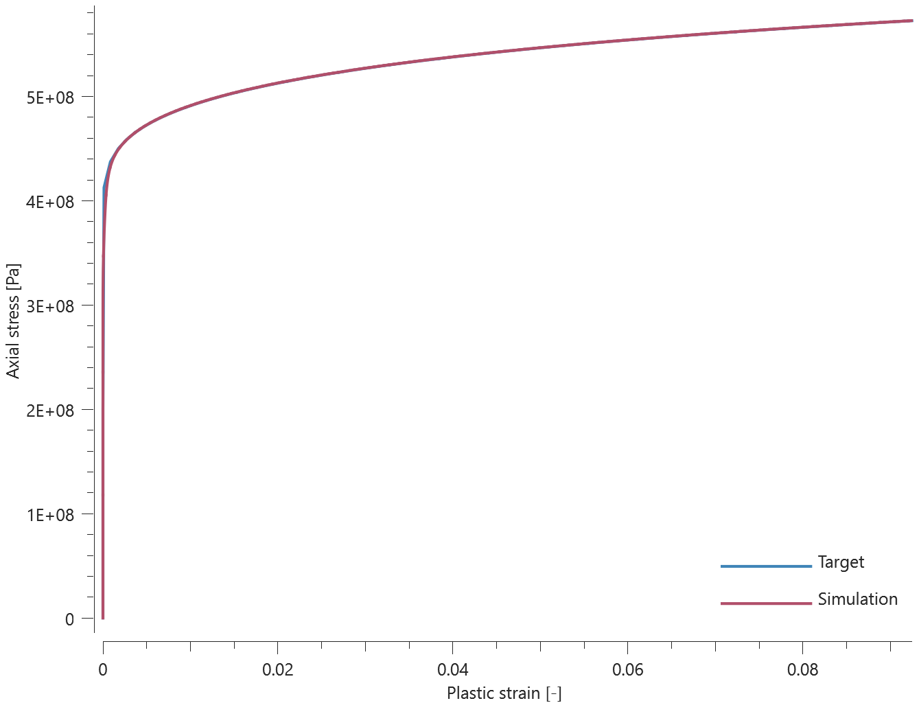
Maximum and average axial stress and plastic strain are checked.
Tests
This benchmark is associated with 1 tests.
*MAT_RIGID
density
"Optional title"
mid, $\rho$, ., ., ., tid
The density in *MAT_RIGID is verified in this test.
Tested parameters: $\rho$.
Maximum and minimum mass of the element are checked.
Tests
This benchmark is associated with 1 tests.
*MAT_VISCOUS_FOAM
Version control
"Optional title"
mid, $\rho$, $E_1$
$\eta$, cid$_{fe}$, cid$_{dec}$, $c_{dec}$, $\sigma_{cut}$, $\gamma$, $\varepsilon_{f}$, $G_{2}$
$\sigma_y$
This test is done for version control of the command *MAT_VISCOUS_FOAM.
A cubic LHEX element is subject for compression. The initial porosity, $\eta$, is set to 0.9 and the compression of the element is done up until 75% of the element length. After the element is compressed 75% the compression stops and the element is expanding up to its initial state.
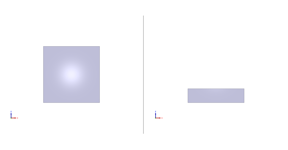
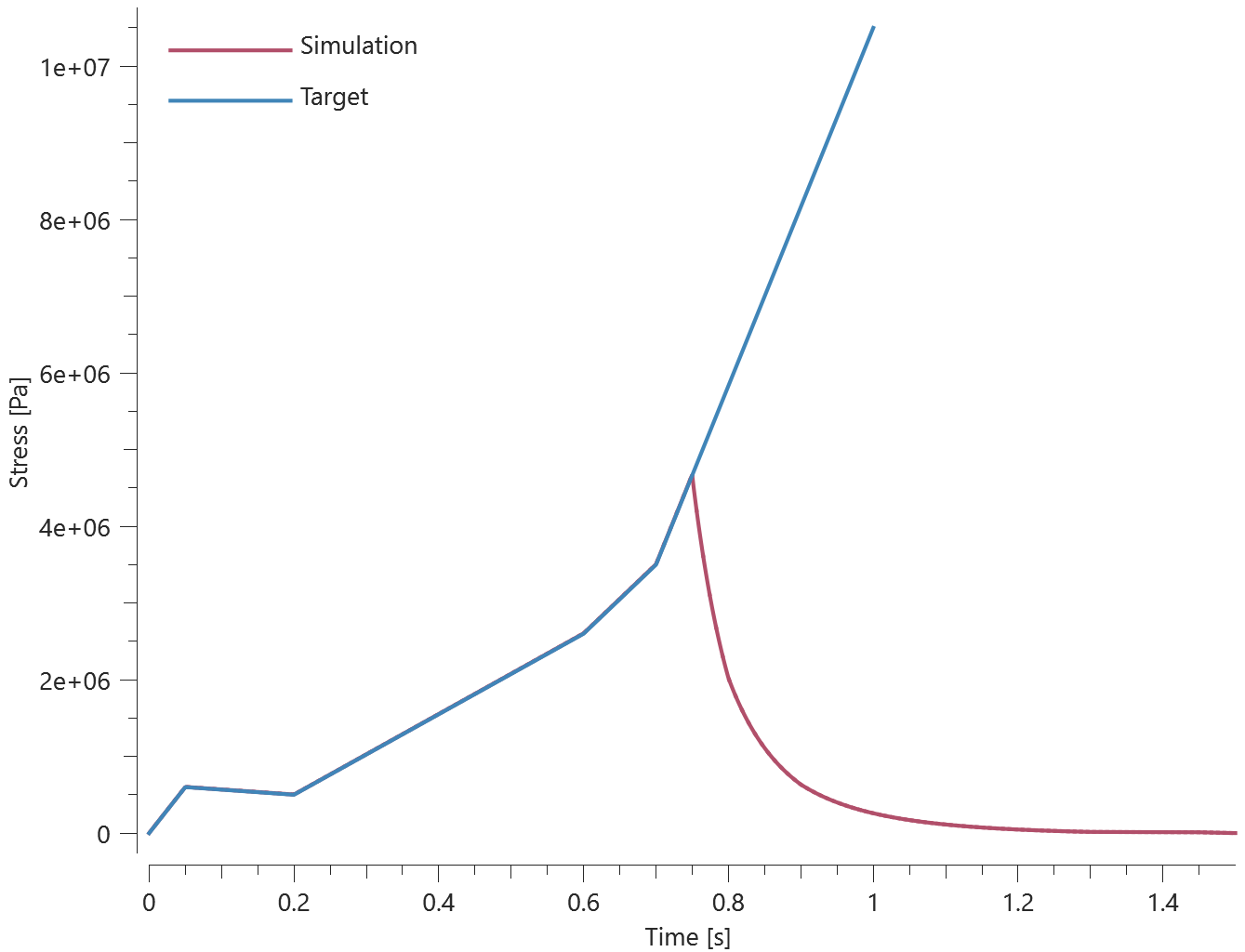
The effective stress and Z-coordinate of the top of the element is checked for verison control.
Tests
This benchmark is associated with 1 tests.
*MAT_VISCO_PLASTIC
Non-linear elasticity
"Optional title"
mid, $\rho$, $E$, $\nu$, did, tid
$\sigma_0$, $Q_1$, $C_1$, $Q_2$, $C_2$, cid, $c_{dec}$, $\alpha$
$\beta$, $m$, $T_0$, $T_m$, $n$
The linear and non-linear elasticity in *MAT_VISCO_PLASTIC are verified in this test.
Tested parameters: $E$, $\nu$, $\alpha$ and $n$.
A CHEX element is stretched in the X-direction while fixed in the Y- and Z-direction. Stress in X-, Y- and Z-direction vs. time are presented in Figure 1 together with target curves from a verification script.
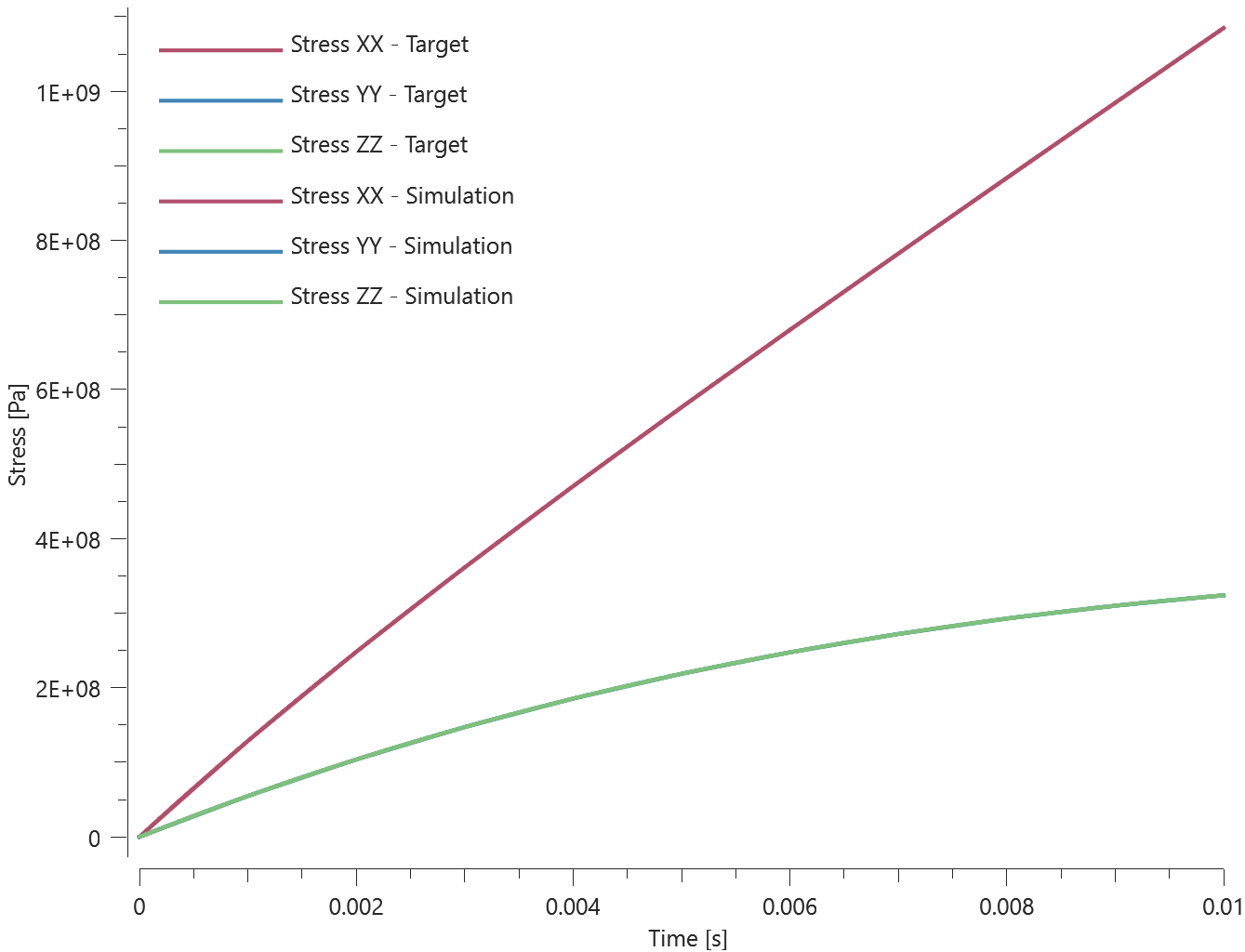
Maximum and average stress in X-, Y- and Z-direction are checked.
Tests
This benchmark is associated with 1 tests.
Plasticity
"Optional title"
mid, $\rho$, $E$, $\nu$, did, tid
$\sigma_0$, $Q_1$, $C_1$, $Q_2$, $C_2$, cid, $c_{dec}$, $\alpha$
$\beta$, $m$, $T_0$, $T_m$, $n$
The plasticity in *MAT_VISCO_PLASTIC is verified in this test.
Tested parameters: $\sigma_0$, $Q_1$, $C_1$, $Q_2$, $C_2$, $\beta$, $m$, $T_0$ and $T_m$.
A CHEX element is loaded in uniaxial tension. Effective stress vs. effective plastic strain and temperature vs. effective plastic strain are presented in Figure 1 and 2 together with target curves from a verification script.
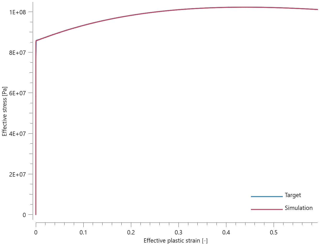
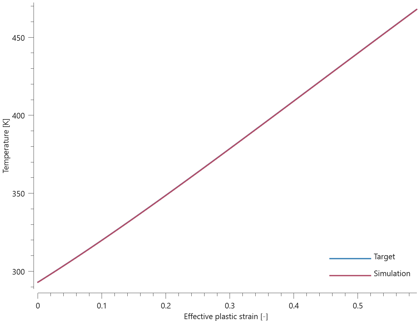
Maximum and average effective stress, temperature and effective plastic strain are checked.
Tests
This benchmark is associated with 1 tests.
Viscosity
"Optional title"
mid, $\rho$, $E$, $\nu$, did, tid
$\sigma_0$, $Q_1$, $C_1$, $Q_2$, $C_2$, cid, $c_{dec}$, $\alpha$
$\beta$, $m$, $T_0$, $T_m$, $n$
The viscosity in *MAT_VISCO_PLASTIC is verified in this test.
Tested parameters: $E$, $\nu$, $cid$ and $c_{dec}$.
A CHEX element is stretched in the X-direction while fixed in the Y- and Z-direction. Stress in X-, Y- and Z-direction vs. time are presented in Figure 1 together with target curves from a verification script.
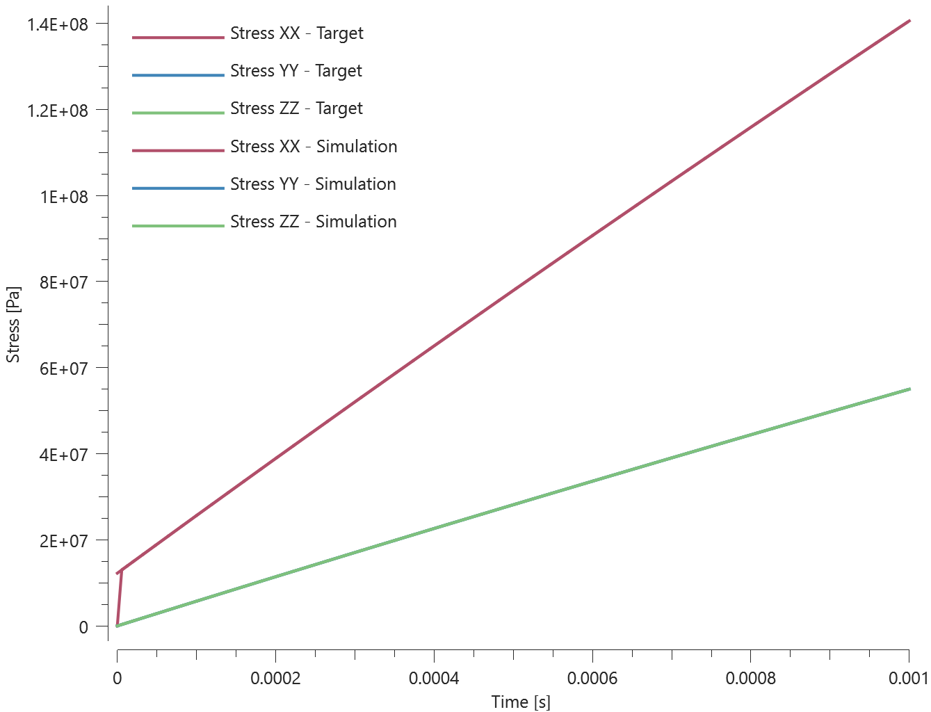
Maximum and average stress in X-, Y- and Z-direction are checked.
Tests
This benchmark is associated with 1 tests.
*MAT_ZA
BCC
"Optional title"
mid, $\rho$, $E$, $\nu$, did, tid, eosid
$\sigma_g$, $k_h$, $l$, $K$, $n$, $B$, $B_0$
$\alpha_0$, $\alpha_1$, $\beta_0$, $\beta_1$, $\dot{\varepsilon}_0$
The athermal part of the flow stress and the BCC-structure parameters of *MAT_ZA is verified in this test.
Tested parameters: $E$, $\nu$, $\sigma_g$, $k_h$, $l$, $K$, $n$, $B$, $\beta_0$, $\beta_1$ and $\dot{\varepsilon}_0$.
A CHEX element is loaded in uniaxial tension. Deformation is caused by a prescribed strain rate. Effective stress vs. effective plastic strain and temperature vs. effective plastic strain are presented in Figure 1 and 2 together with target curves from a verfication script.
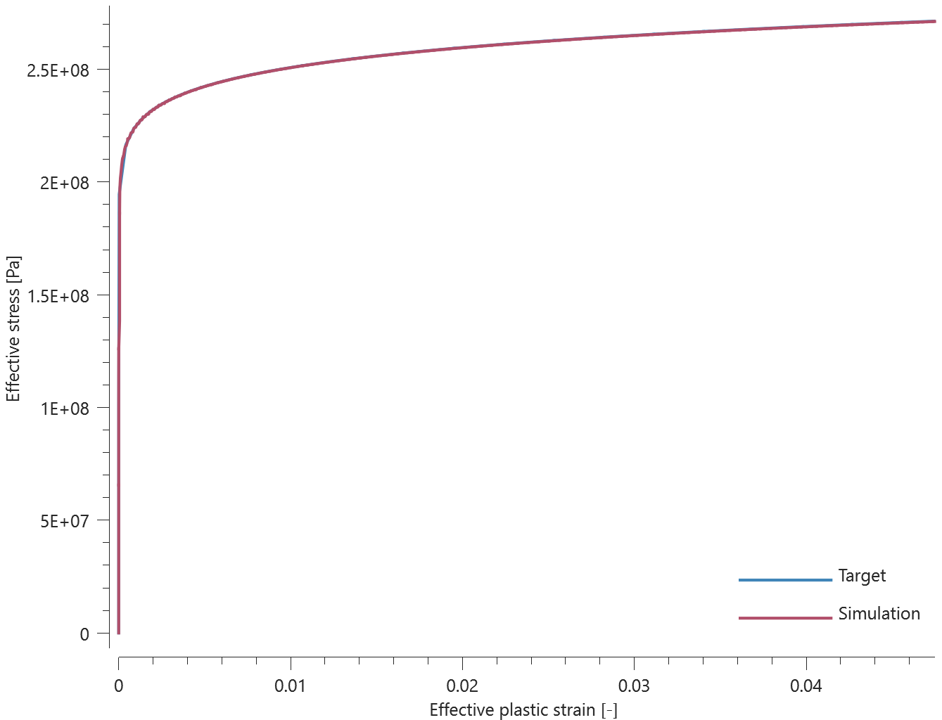
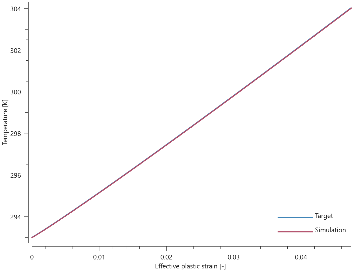
Maximum and average effective stress, effective plastic strain and temperature are checked.
Tests
This benchmark is associated with 1 tests.
FCC
"Optional title"
mid, $\rho$, $E$, $\nu$, did, tid, eosid
$\sigma_g$, $k_h$, $l$, $K$, $n$, $B$, $B_0$
$\alpha_0$, $\alpha_1$, $\beta_0$, $\beta_1$, $\dot{\varepsilon}_0$
The athermal part of the flow stress and the FCC-structure parameters of *MAT_ZA is verified in this test.
Tested parameters: $E$, $\nu$, $\sigma_g$, $k_h$, $l$, $K$, $n$, $B_0$, $\alpha_0$, $\alpha_1$ and $\dot{\varepsilon}_0$.
A CHEX element is loaded in uniaxial tension. Deformation is caused by a prescribed strain rate. Effective stress vs. effective plastic strain and temperature vs. effective plastic strain are presented in Figure 1 and 2 together with target curves from a verification script.
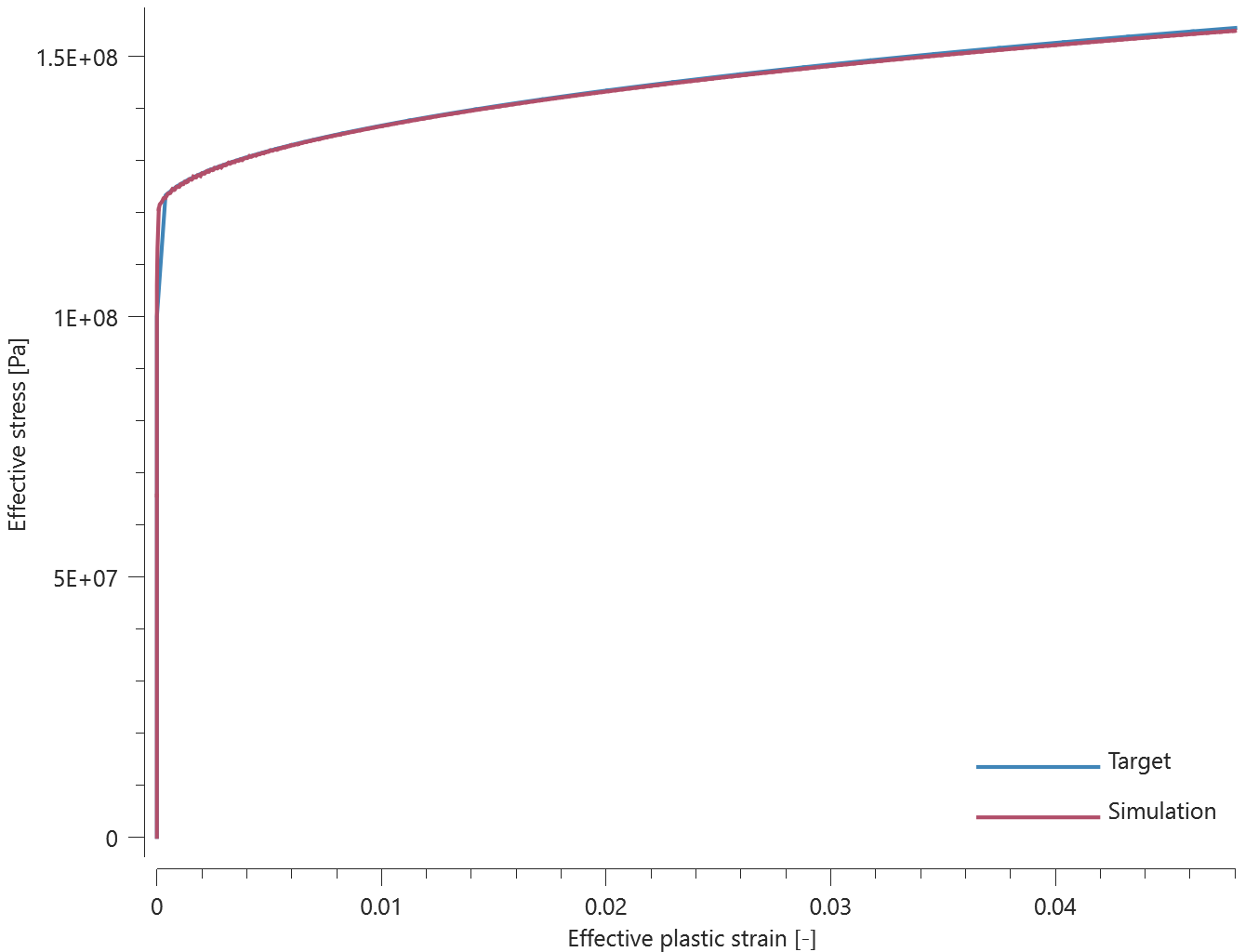
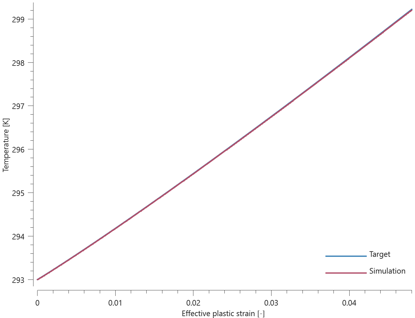
Maximum and average effective stress, effective plastic strain and temperature are checked.
Tests
This benchmark is associated with 1 tests.
*MERGE
All element types
"Optional title"
coid
entype${}_s$, enid${}_s$, entype${}_m$, enid${}_m$, $tol$, mfid, gid, penalty, $\alpha_{max}$, no_self
This tests the *MERGE command. The set-up is nine bottom plates of one element type that are merged to nine smaller top plates. The bottom plates are of one element type, while the smaller top plates covers the other nine element types, as seen in Figure 1. Throughout nine tests, all nine element types (linear/quadratic/cubic, hexahedron/pentahedron/tetrahedron) are checked as both bottom plate and top plate. Nine tests of nine plate-pairs give 81 merge operations to check.

The plates are merged using the *MERGE command, after which they are exposed to tensile and sheer forces. *LOAD_FORCE is applied in both X- and Z-direction with a smooth curve function that reach $1 \ MPa$ just before termination time. Forces in X- and Z-direction are output to "merge.out", so is the total force (target: $\sqrt2 \ MPa$). These values are used for version control. Plots of the total force curves for all 81 plate-pairs are shown in Figure 2 - Figure 10.

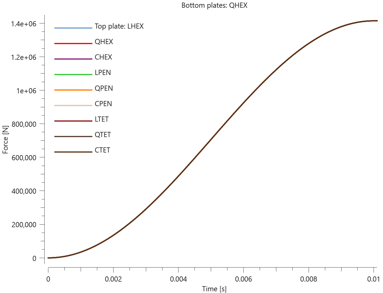

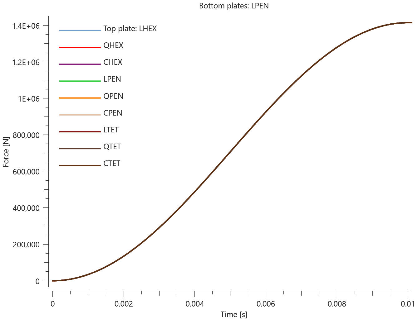
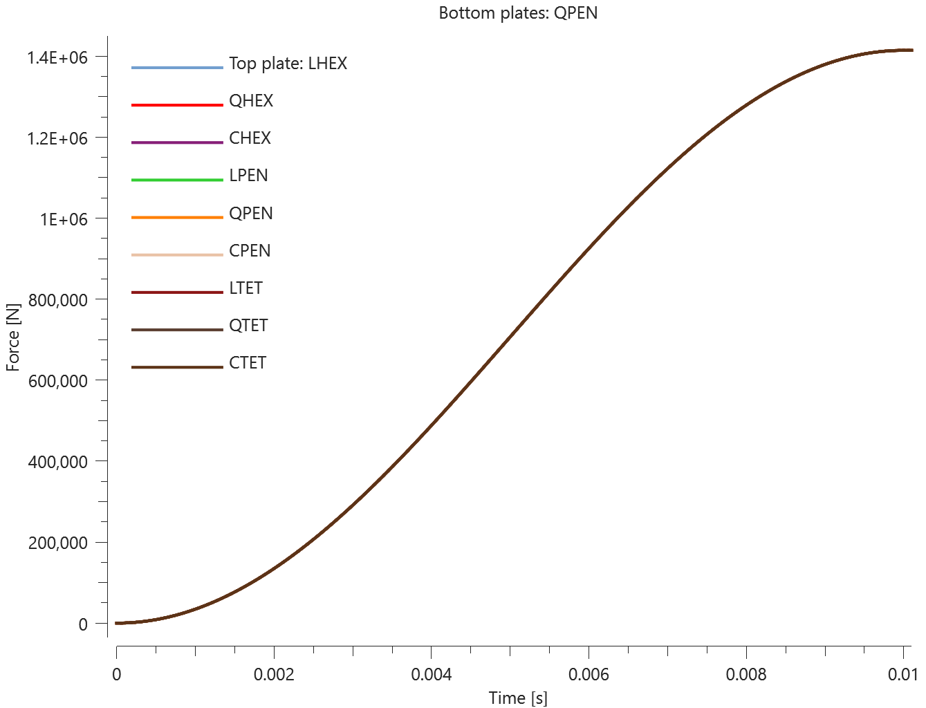


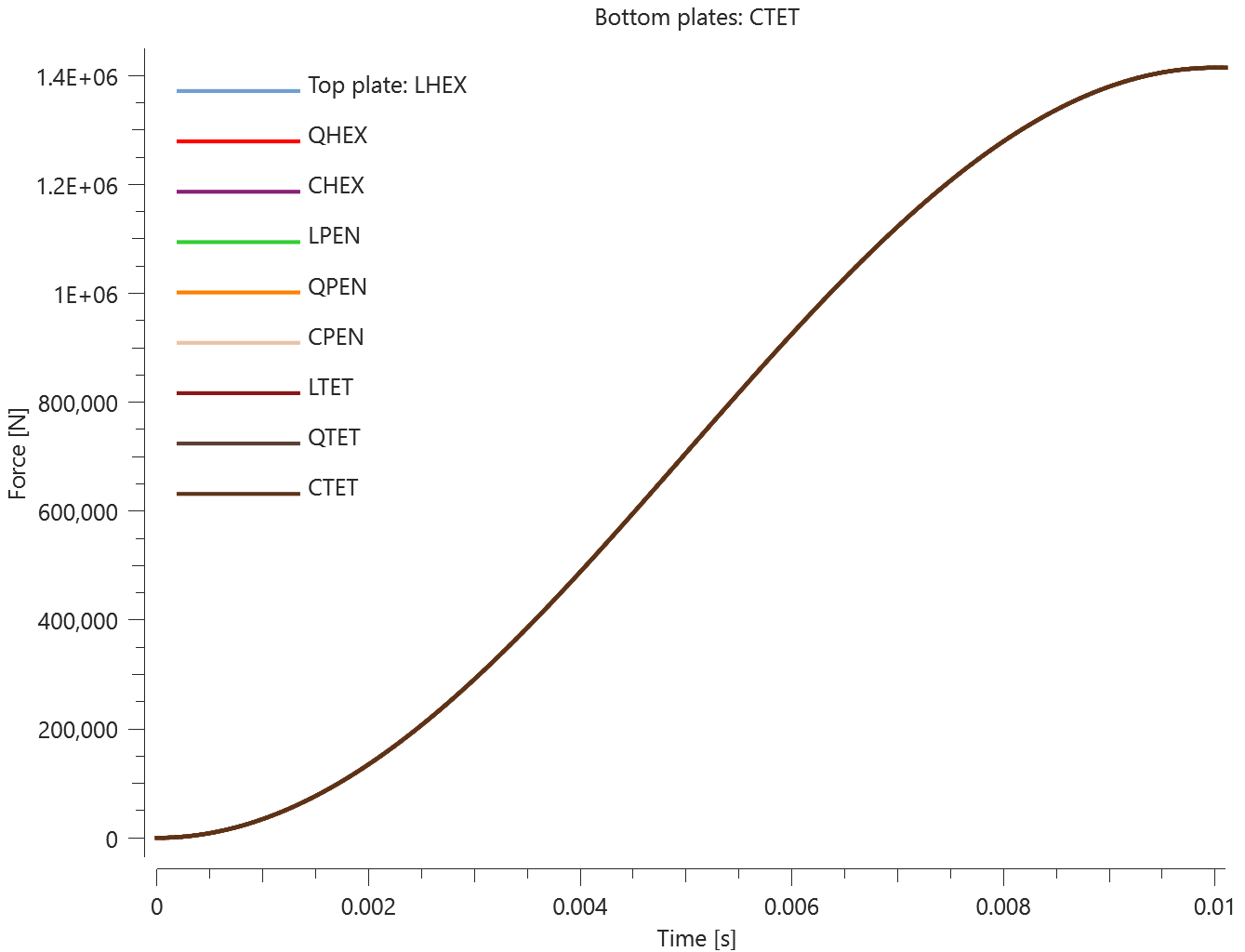
Tests
This benchmark is associated with 9 tests.
Initial displacements
"Optional title"
coid
entype${}_s$, enid${}_s$, entype${}_m$, enid${}_m$, $tol$, mfid, gid, penalty, $\alpha_{max}$, no_self
This model tests automatic generation of initial displacements when using the command *MERGE. A pipe (slave entity) is merged to a plate (master entity). The pipe is slightly tilted so that the surfaces of the parts that will be merged are not perpendicular.
In step 1, the solver is initiated. The file: _node_merge_project.k is automatically generated when starting a simulation with the command *MERGE. It contains the initial displacement projection vectors for all merged slave nodes.
In step 2, the file containing the initial displacements is included to the main file. The node positions of the slave nodes are adjusted when rerun.
It is checked whether the merge is completed succesfully for version control.
Tests
This benchmark is associated with 2 tests.
Multistep merge
"Optional title"
coid
entype${}_s$, enid${}_s$, entype${}_m$, enid${}_m$, $tol$, mfid, gid, penalty, $\alpha_{max}$, no_self
This model tests the automatic generation of merging nodes to faces when using the command *MERGE in multiple step simulations.
The test consists of 3 steps. Two plates are merged. The upper plate is fixed in space while the lower plate is subjected to gravity. Parameter entype_res is set to ALL in *OUTPUT for step 1, 2 & 3. The command *MERGE is only used in the first step. If working as intended the lower plate should not fall do to gravity.
In step 1, the command *MERGE will output the *MERGE_NODE_TO_FACE commands in the output file impetus_state_merge1.k at termination.
In step 2, The file impetus_state_merge1.k is included from step 1 to the model. *MERGE does not need to be used again.
In step 3, The *MERGE_NODE_TO_FACE commands will now be located in the file impetus_state1.k from step 2 which is included in this step.
It is checked that both plates remain at their initial positions for version control.
Tests
This benchmark is associated with 3 tests.
Parallelism
"Optional title"
coid
entype${}_s$, enid${}_s$, entype${}_m$, enid${}_m$, $tol$, mfid, gid, penalty, $\alpha_{max}$, no_self
Tested parameters: $entype_s$, $enid_s$, $entype_m$, $enid_m$, $tol$, $\alpha_{max}$.
This model tests the parameter $\alpha_{max}$ for the command *MERGE. The parameter can be used to control the maximum allowed deviation from parallelism. The test consists of four components that are close to but not parallell to a fifth component, with an increasing discrepancy in parallelism, varying in the range of 5° to 45°. See Figure 1.
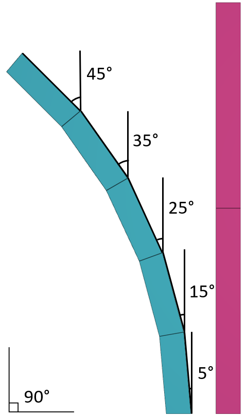
The four components consisting of 5 elements each, are merged to the fifth component. The parameter $\alpha_{max}$ has a default value of 25° which is instead set to 6°, 16°, 26° and 36° for the different parts. An erode condition is set to the elements that exceeds these angles for the respective parts. See Figure 2.
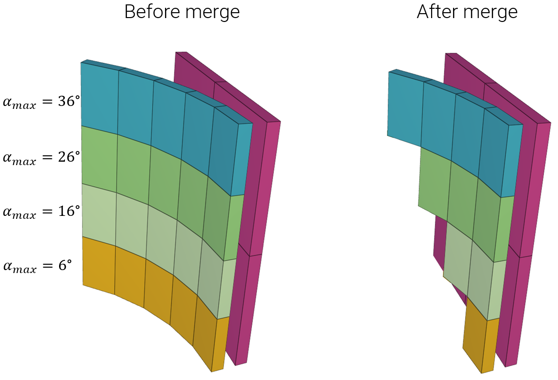
It is checked whether the merge is completed succesfully in version control.
Tests
This benchmark is associated with 1 tests.
*MERGE_DUPLICATED_NODES
Merge and load force
entype${}_s$, enid${}_s$, entype${}_m$, enid${}_m$, $tol$
This tests the *MERGE_DUPLICATED_NODES command. It consists of eight rigid bodies created by the *COMPONENT_CYLINDER command. The bodies are lined up in pairs. The first set consists of two identical and perfectly overlapping bodies. In the second set the bodies have different mesh densities, but still perfectly overlaps. In the third and fourth sets the bodies are identical but at distances $0.10$ and $0.12$, respectively, apart from each other.
The first two sets are merged with a tolerance of $1e^{-6}$, and the last two sets with a tolerance of $0.11$. Only the first three sets should thus be successfully merged. LOAD_PRESSURE is then applied to check that the bodies react appropriately. Expected accelerations is listed in the Table 1.
| Part ID | Set | Rigid body ID $(After \ merge)$ | Mass $(kg)$ | Applied force $(N)$ | Exp. Acceleration $(m/s^2)$ |
|---|---|---|---|---|---|
| 1 2 |
1 | 1 | $1.20\cdot10^4$ | $1\cdot10^4$ | 0.833 |
| 3 4 |
2 | 3 | $1.18\cdot10^4$ | $1\cdot10^4$ | 0.842 |
| 5 6 |
3 | 5 | $1.20\cdot10^4$ | $1\cdot10^4$ | 0.833 |
| 7 8 |
4 | 7 8 |
$6.00\cdot10^4$ $5.64\cdot10^4$ |
$1 \cdot 10^4$ 0 |
1.677 |
The results are checked against "rigid.out"
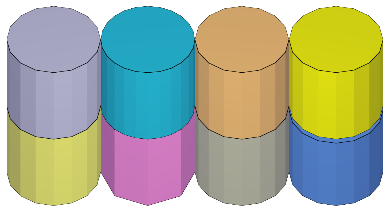
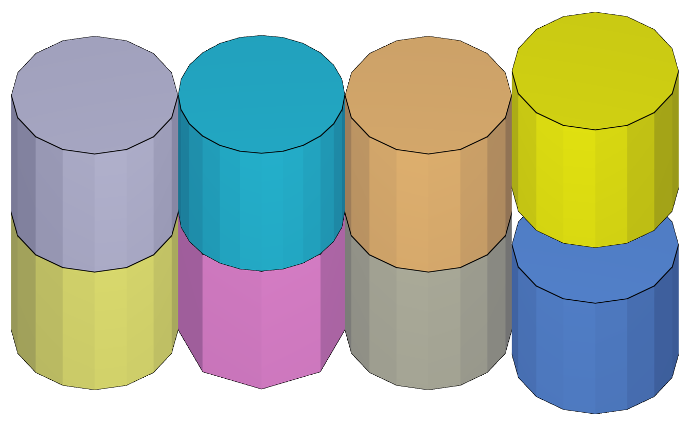
Tests
This benchmark is associated with 1 tests.
*MERGE_FAILURE_COHESIVE
Normal stress
mfid, $\sigma_{fail}$, $\tau_{fail}$, $G_{I}$, $G_{II}$, $\Delta_{ref}$
Two quadratic plates with side length, $L$, and thickness, $t$, are merged as displayed in Figure 1. The plates are modeled as elastic with a Young's modulus, $E$, and a Poisson's ratio, $\nu$. A prescribed displacement is imposed on the plates, causing a state of normal stress in the merge.
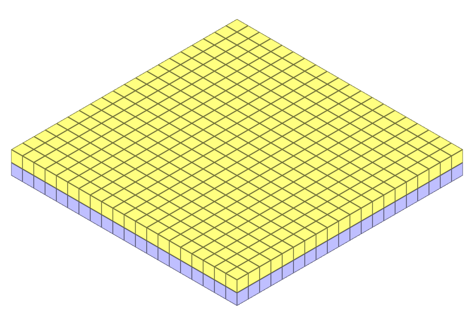
Given the tensile failure stress, $\sigma_{fail}$, defined in this test, the stress should reach the tensile failure stress at a displacement, $\delta$:
$$ \delta = \sigma_{fail} \cdot 2 \cdot t/E $$
In this test, complete failure is to occur at a displacement of $2 \cdot \delta$.
Energy, $W$, consumed at complete failure:
$$ W = \sigma_{fail} \cdot L^2 \cdot \delta $$
Energy per unit area, $G$, consumed at complete failure:
$$ G = W/L^2 $$
The prescribed displacement is defined as $2 \cdot \delta$, and the modus I energy per unit area is defined as $G$. Force vs displacement from the simulation is presented in Figure 2 and 3 together with a target curve based on the calculations above. The test is done with both constraint and penalty based merge (defined in *MERGE).
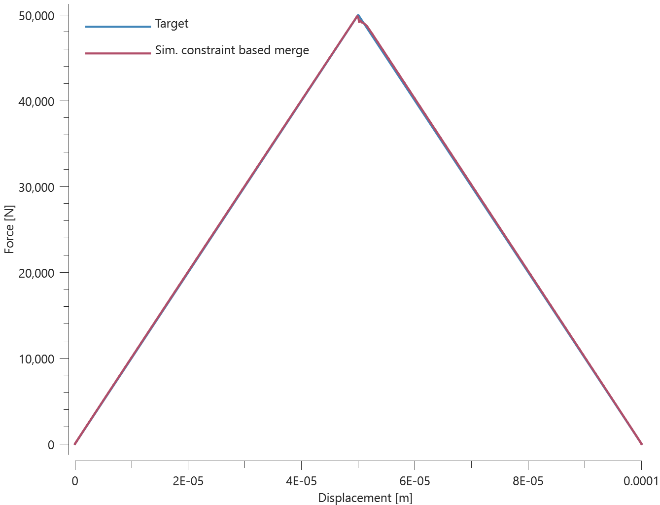
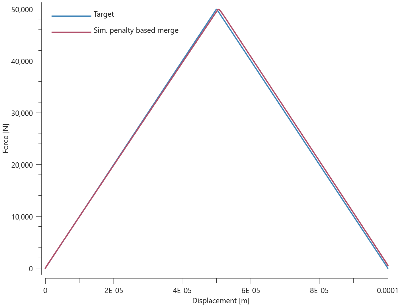
Max and average force and max displacement is checked for both the constraint and penalty based merge.
Tests
This benchmark is associated with 2 tests.
Shear stress
mfid, $\sigma_{fail}$, $\tau_{fail}$, $G_{I}$, $G_{II}$, $\Delta_{ref}$
This test is similar to the test "*MERGE_FAILURE_COHESIVE - Normal stress". In the current test, the merge is subjected to a state of shear stress instead.
Given the shear failure stress, $\tau_{fail}$, defined in this test, the stress should reach the shear failure stress at a displacement, $\delta$:
$$ \delta = tan\left(\tau_{fail} \cdot 2\cdot(1+\nu)/E\right) \cdot 2 \cdot t $$
In this test, complete failure is to occur at a displacement of $2 \cdot \delta$.
Energy, $W$, consumed at complete failure:
$$ W = \tau_{fail} \cdot L^2 \cdot \delta $$
Energy per unit area, $G$, consumed at complete failure:
$$ G = W/L^2 $$
The prescribed displacement is defined as $2 \cdot \delta$, and the modus II energy per unit area is defined as $G$. Force vs displacement from the simulation is presented in Figure 1 and 2 together with a target curve based on the calculations above. The test is done with both constraint and penalty based merge (defined in *MERGE).
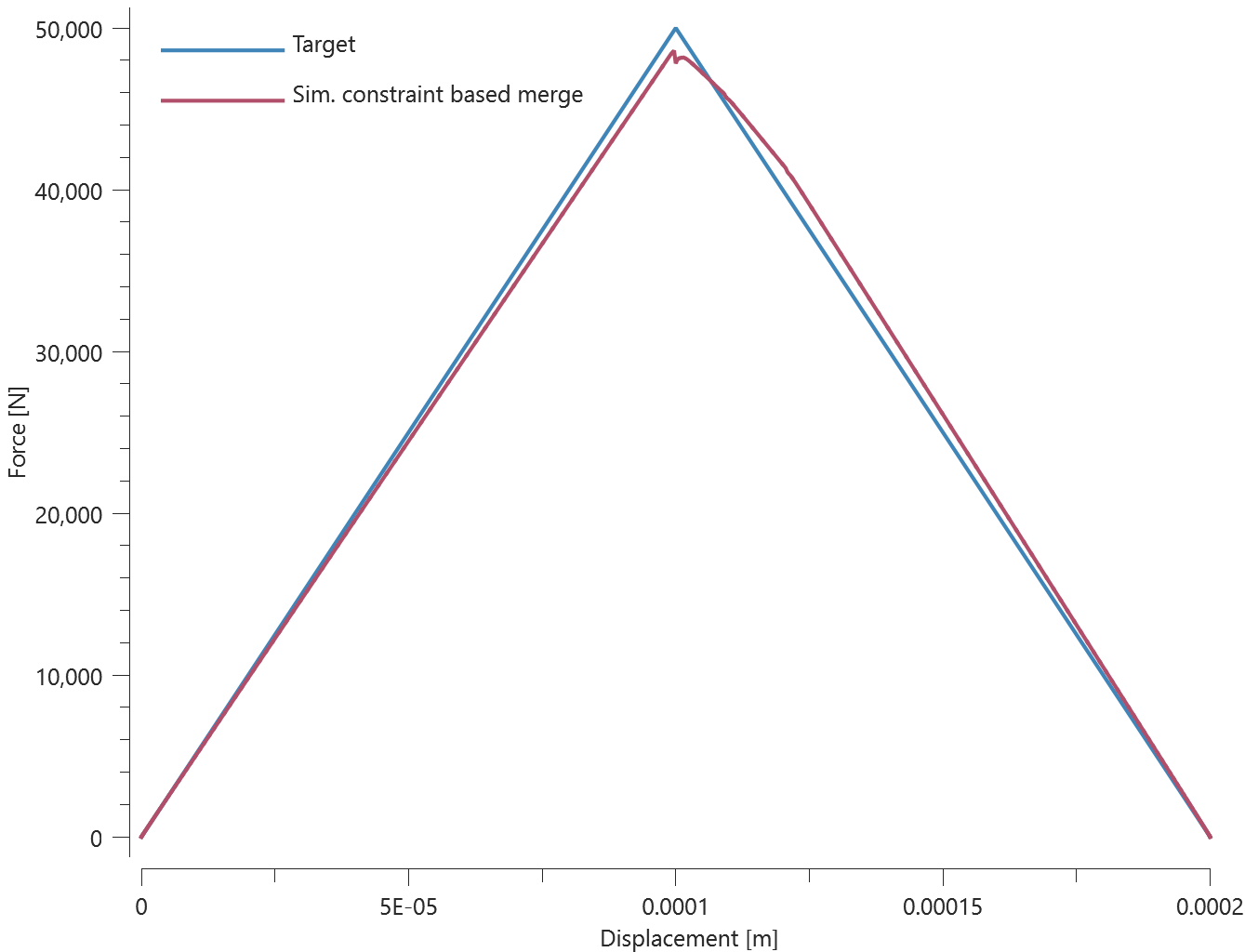
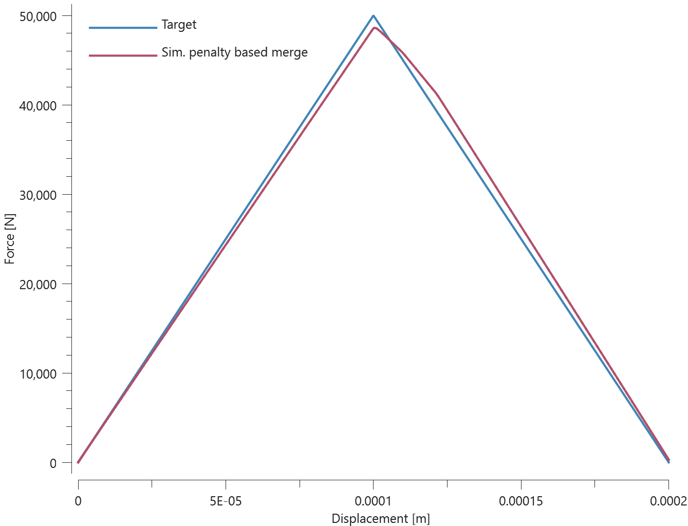
Max and average force and max displacement is checked for both the constraint and penalty based merge.
Tests
This benchmark is associated with 2 tests.
*MERGE_FAILURE_FORCE
Failure exponents
mfid, $T_{fail}$, $S_{fail}$, $n_T$, $n_S$
Tested parameters: mfid, $T_{fail}$, $S_{fail}$, $n_T$, $n_S$.
This model tests the tensile- & shear failure exponents in the *MERGE_FAILURE_FORCE command. Two components are merged togheter. A combination of tensile and shear forces are introduced to one of the components. The merge failure condition is set to:
- Tensile failure force, $T_{fail}=100 \ N$
- Shear failure force, $S_{fail}=100 \ N$
- Tensile failure exponent, $n_{T}=1$
- Shear failure exponent, $n_{S}=1$
Target:
The merge forces (merge.out) should sum up to 100 N at failure: $F_x + F_z = 100 \ N$
Tests
This benchmark is associated with 1 tests.
Shear and tensile failure
mfid, $T_{fail}$, $S_{fail}$, $n_T$, $n_S$
This tests the *MERGE_FAILURE_FORCE command against combined shear- and tensile forces. As in the *MERGE benchmark, the set-up is nine bottom plates of one element type that are merged to nine smaller top plates, se seen in Figure 1. Each merge is given a failure condition with the *MERGE_FAILURE_FORCE command. Tensile- and shear failure forces are specified at $2e^{6} \ N$. In this test, the plates are exposed to an equal shear- and tensile force.
A force surpassing failure criteria is applied. The bottom plates are of one element type, while the top plates covers the other nine element types. Throughout nine tests, all nine element types (linear/quadratic/cubic, hexahedron/pentahedron/tetrahedron) are checked as both bottom plate and top plate. Nine tests of nine plate-pairs give 81 merge operations to check.

*LOAD_FORCE is applied in X- and Z-direction on the top plates with a smooth curve function. Bottom plates are held in place with *BC_MOTION. The force between the plates in each direction is output to "merge.out" for all plate-pairs. These values are used for version control. Plots of the total force curves for all 81 plate-pairs are shown in Figure 2 - 10.
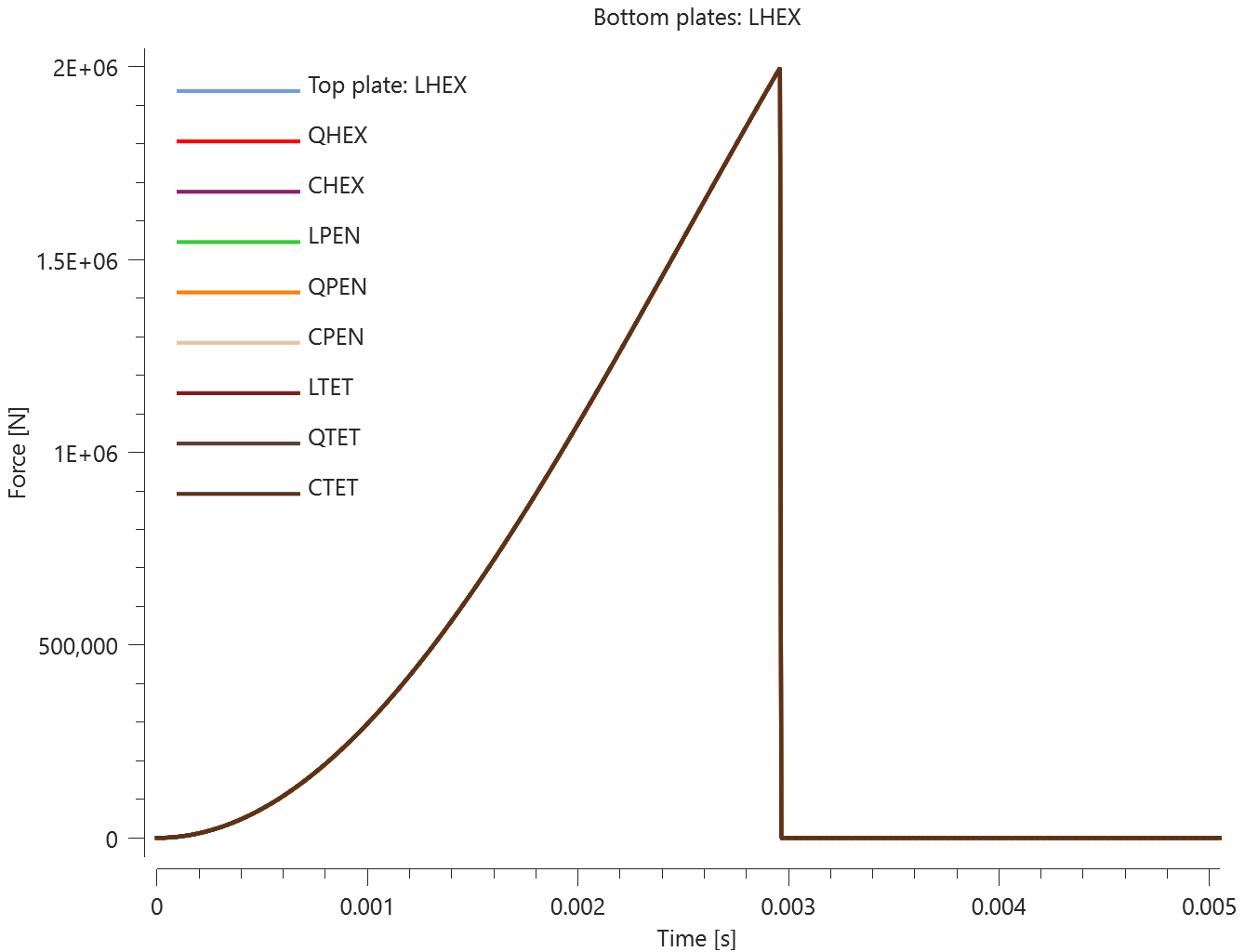
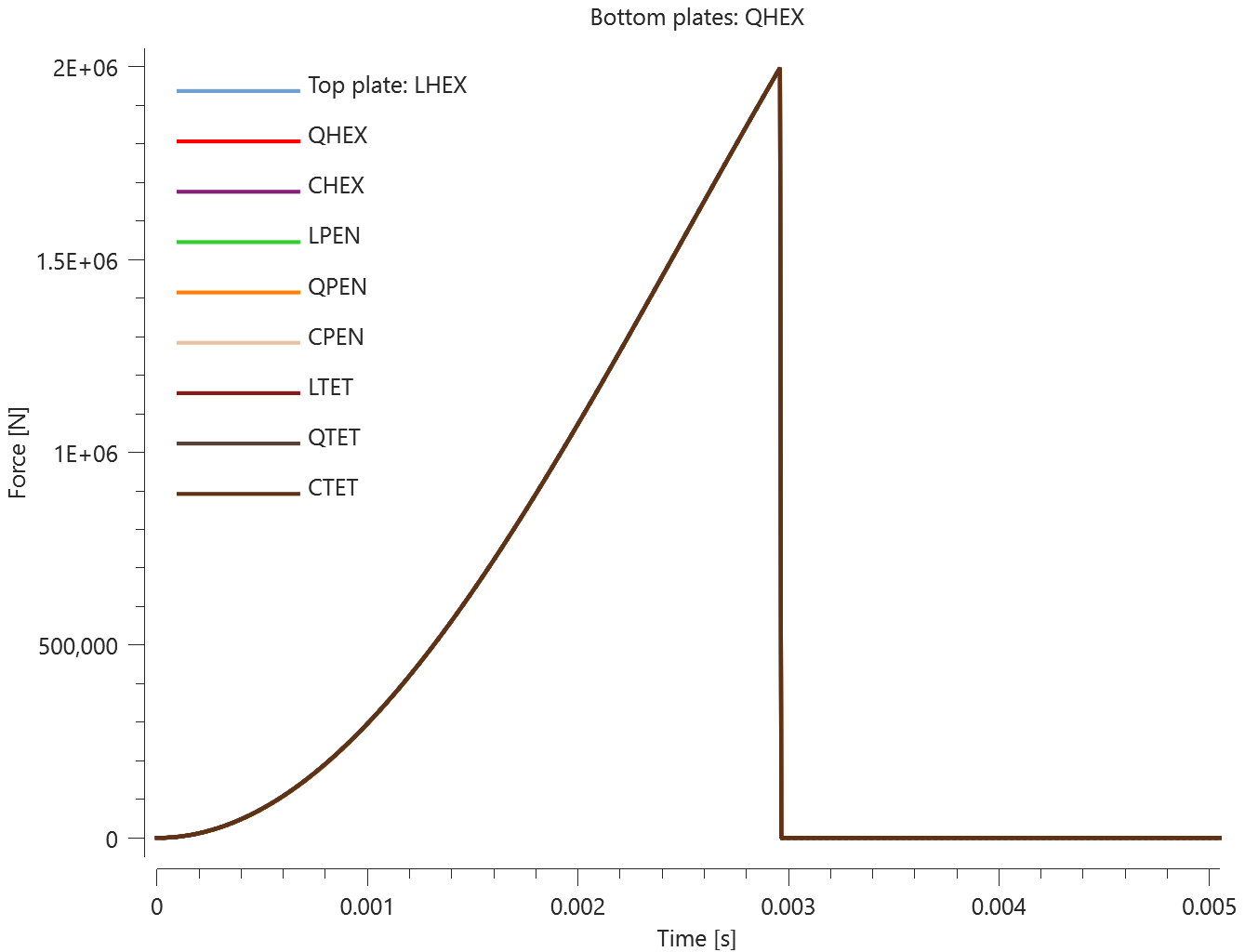

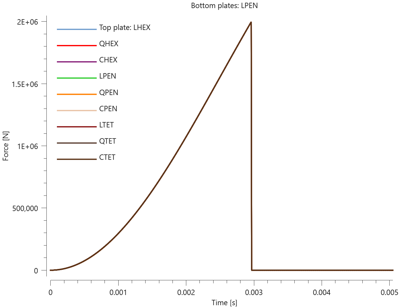


Tests
This benchmark is associated with 9 tests.
Shear failure
mfid, $T_{fail}$, $S_{fail}$, $n_T$, $n_S$
This tests the *MERGE_FAILURE_FORCE command against a shear force. As in the *MERGE benchmark, the set-up is nine bottom plates of one element type that are merged to nine smaller top plates, as seen in Figure 1. Each merge is given a failure condition with the *MERGE_FAILURE_FORCE command. Tensile- and shear failure forces are specified at $2e^{6} \ N$. In this test, the plates are exposed to a shear force only.
A force surpassing failure criteria is applied. The bottom plates are of one element type, while the top plates covers the other nine element types. Throughout nine tests, all nine element types (linear/quadratic/cubic, hexahedron/pentahedron/tetrahedron) are checked as both bottom plate and top plate. Nine tests of nine plate-pairs give 81 merge operations to check.

*LOAD_FORCE is applied in X-direction on the top plates with a smooth curve function. Bottom plates are held in place with *BC_MOTION. The force between the plates in X-direction is output to "merge.out" for all plate-pairs. These values are used for version control. Plots of the total force curves for all 81 plate-pairs are shown in Figure 2 - 10.


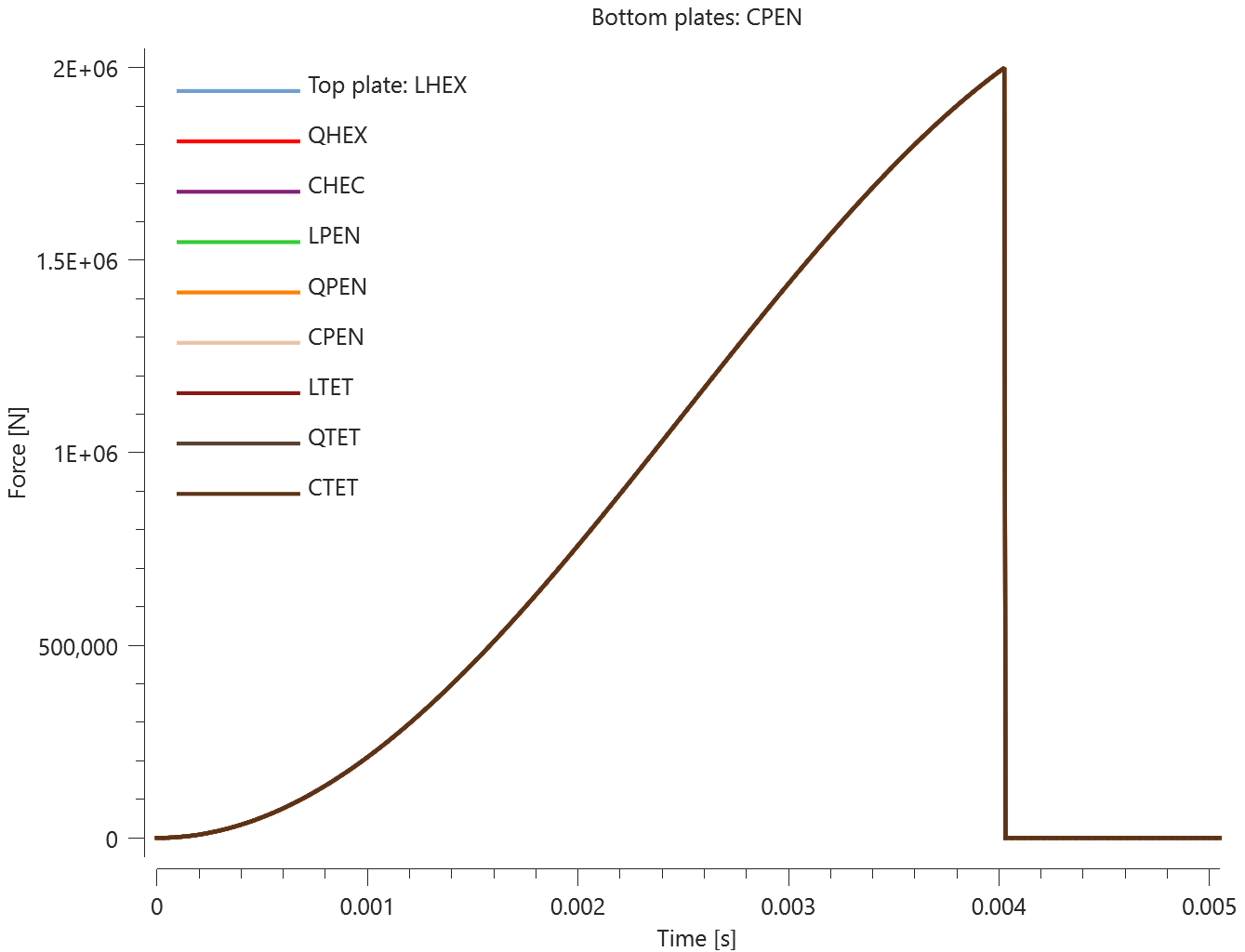


Tests
This benchmark is associated with 9 tests.
Tensile failure
mfid, $T_{fail}$, $S_{fail}$, $n_T$, $n_S$
This tests the *MERGE_FAILURE_FORCE command against a tensile force. As in the *MERGE benchmark, the set-up is nine bottom plates of one element type that are merged to nine smaller top plates, as seen in Figure 1. Each merge is given a failure condition with the *MERGE_FAILURE_FORCE command. Tensile- and shear failure forces are specified at $2e^{6} \ N$. In this test, the plates are exposed to a tensile force only.
A force surpassing failure criteria is applied. The bottom plates are of one element type, while the top plates covers the other nine element types. Throughout nine tests, all nine element types (linear/quadratic/cubic, hexahedron/pentahedron/tetrahedron) are checked as both bottom plate and top plate. Nine tests of nine plate-pairs give 81 merge operations to check.
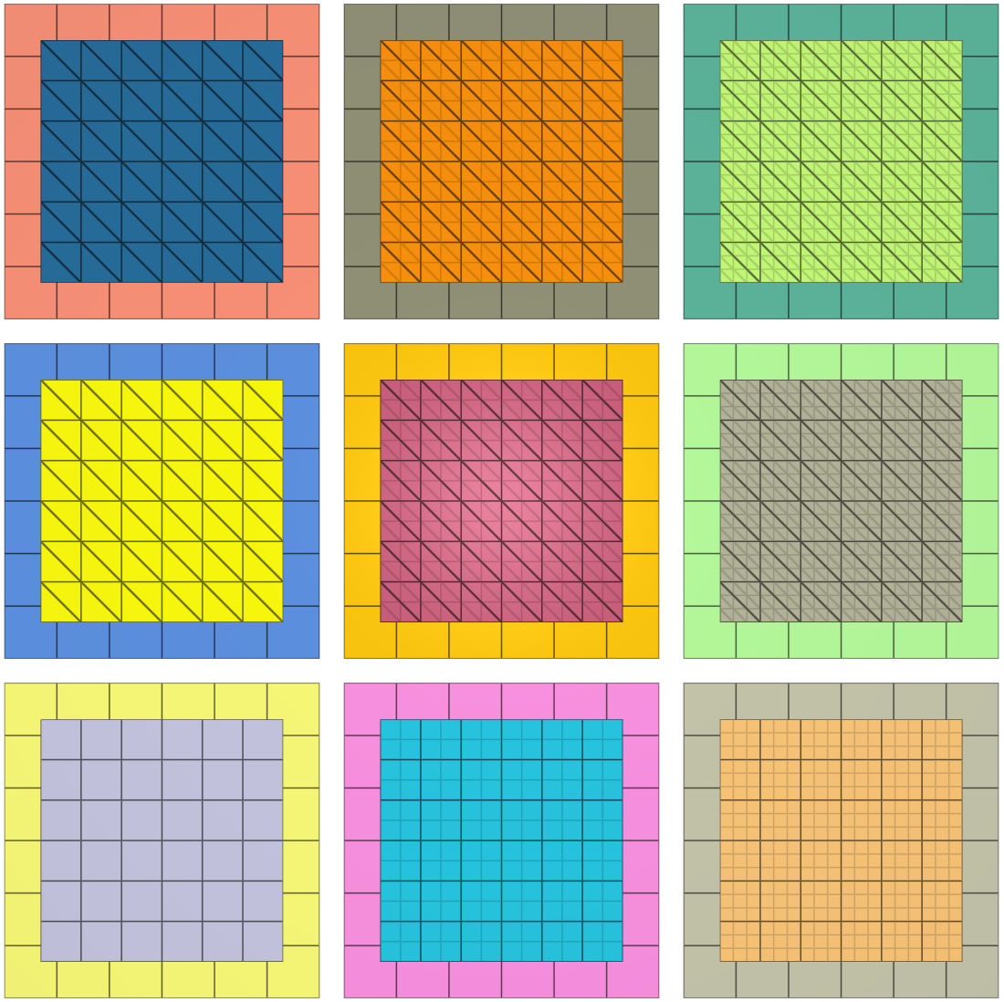
*LOAD_FORCE is applied in Z-direction on the top plates with a smooth curve function. Bottom plates are held in place with *BC_MOTION. The force between the plates in Z-direction is output to "merge.out" for all plate-pairs. These values are used for version control. Plots of the total force curves for all 81 plate-pairs are shown in Figure 2 - 10.


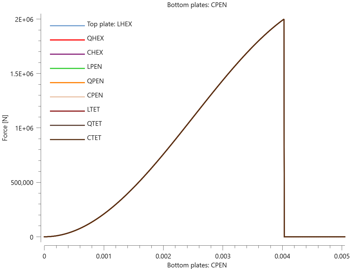


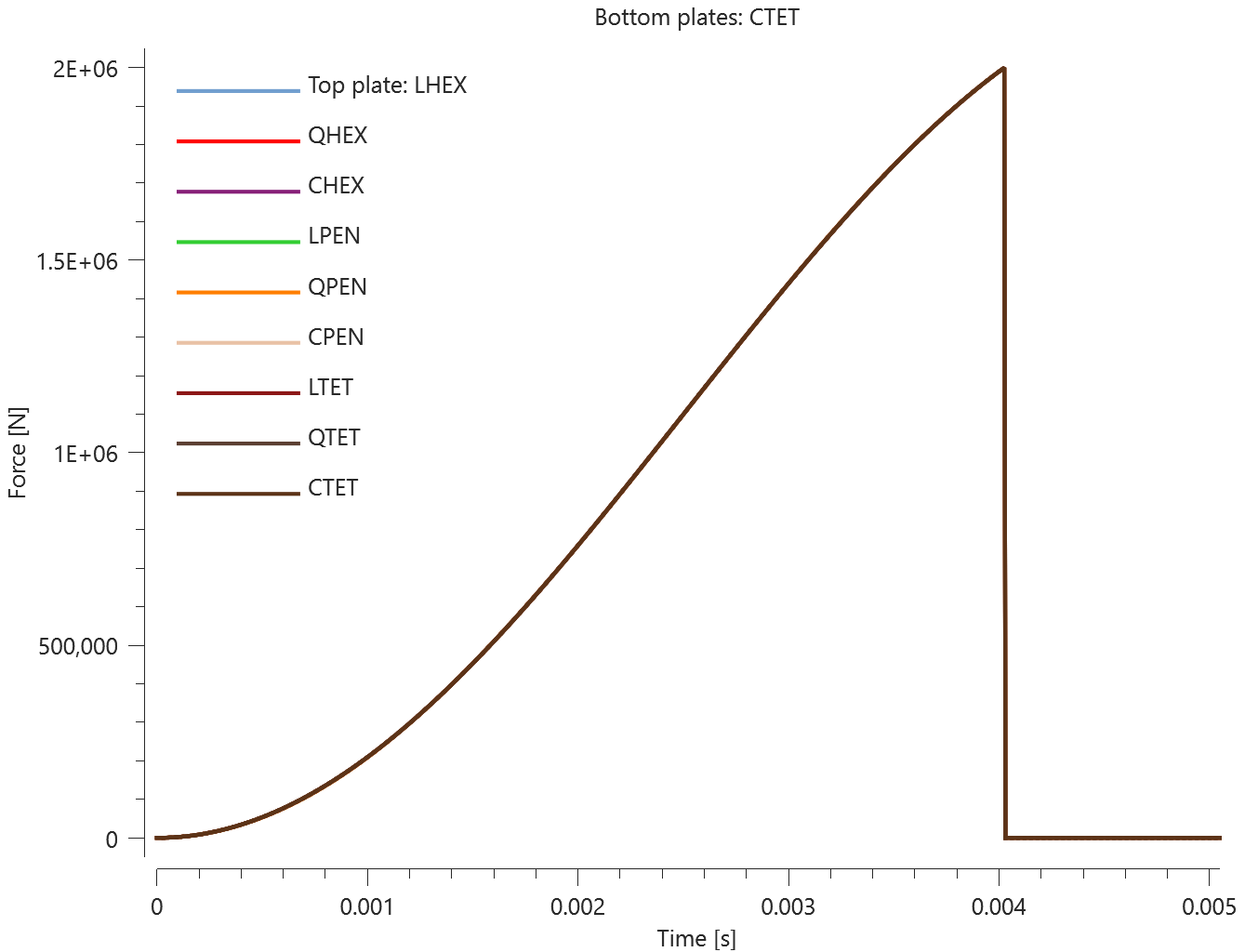
Tests
This benchmark is associated with 9 tests.
*NODE
Coordinates
nid, $x$, $y$, $z$, bc
This tests the *NODE command. A simple solid element is meshed using *NODE and *ELEMENT_SOLID. The volume and physical mass is checked to test that all the nodes are correctly generated.
Tests
This benchmark is associated with 1 tests.
*OUTPUT_CONTACT_FORCE
Two colliding spheres
"Optional title"
coid, entype, enid
Tested parameters: coid, entype, enid.
This model tests the *OUTPUT_CONTACT_FORCE command. Two spheres are colliding. With *OUTPUT_CONTACT_FORCE, it is possible to specify a region where all the contact forces are sampled and output to the ASCII file contact_force.out.
The test setup is displayed in Figure 1.
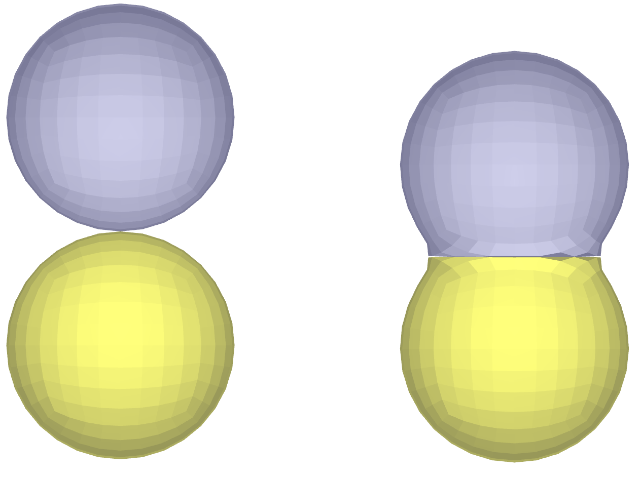
In total, eight outputs are generated for verification. This can be seen in Figure 2
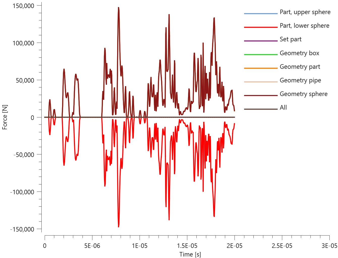
Targets:
- Part, Upper sphere. Maximum contact force Z-component = 148130 N
- Part, Lower sphere. Minimum contact force Z-component = -148130 N
- Set part. Maximum contact force Z-component = 0 N
- Geometry Box. Maximum contact force Z-component = 148130 N
- Geometry Part. Maximum contact force Z-component = 148130 N
- Geometry Pipe. Maximum contact force Z-component = 148130 N
- Geometry Sphere. Maximum contact force Z-component = 148130 N
- All. Maximum contact force Z-component = 0 N
Tests
This benchmark is associated with 1 tests.
*OUTPUT_DEBUG
User-defined debug information
entype, enid
This model tests the command *OUTPUT_DEBUG. A number of cubes are generated with *COMPONENT_BOX and with the ~repeat command. There is maximum allowed coordinate, $x0=1.8$. A debug command is added to warn if this limit is exceeded.
It is tested that the debug message is displayed in the impetus.info file.
Tests
This benchmark is associated with 1 tests.
*OUTPUT_ELEMENT
Element output
entype, enid
This tests the *OUTPUT_ELEMENT command. A single linear hexahedron element is stretched using *BC_MOTION. *PROP_DAMAGE_CL is used to investigate damage output. The following outputs are checked in the file element.out:
| Stress XX | Stress YY | Stress ZZ |
| Stress XY | Stress YZ | Stress ZX |
| Strain XX | Strain YY | Strain ZZ |
| Strain XY | Strain YZ | Strain ZX |
| Volume | Plastic strain | Damage |
The element is stretched in the Z-direction, but to account for noise a tolerance of $1e7$ relative to zero is allowed for stress in the other directions.
Tests
This benchmark is associated with 1 tests.
*OUTPUT_FORMING
Thickness output
form
This tests the *OUTPUT_FORMING command. The command outputs the thickness through an element. A single cubic hex element is stretched with a velocity function in *BC_MOTION. Integrating the velocity function over simulation time frame gives a total displacement of $1.7$ times the original side length. Final thickness is checked for version control.
Tests
This benchmark is associated with 1 tests.
*OUTPUT_NODE
Node output
entype, enid
This tests the *OUTPUT_NODE command. A single linear hexahedron element is put in motion using *BC_MOTION, *INITIAL_VELOCITY, and *LOAD_FORCE. The element moves along the X-axis. It also rotates about the X-axis, which runs through its center. Set-up conditions are listed below:
$$ V = 1 \ m^3 $$ $$ \rho = 1000 \ kg/m^3 $$ $$ V_{x_0} = 2 \ m/s $$ $$ \omega_{x_0} = 4\pi \ rad/s $$ $$ F_x = -8000 \ N $$ $$ t_{end} = 0.5 \ s $$
| Entity | Value | Analytical expression | Target |
|---|---|---|---|
| X-coordinate | last value | $ x = v_{x_0}t + \dfrac{1}{2}\left(\dfrac{F}{m}\right)t^2$ | $x_{end} = x_{0}$ |
| Y-coordinate | last value | $ 4 \pi rads^{-1} \cdot 0.5 s = 1 rev$ | $y_{end} = y_{0}$ |
| Z-coordinate | last value | $ 4 \pi rads^{-1} \cdot 0.5 s = 1 rev$ | $z_{end} = z_{0}$ |
| X-displacement | max | $0.25 \ m$ | |
| Y-displacement | min/max | $\sqrt{0.5}$ | $\pm 0.707 m$ |
| Z-displacement | min/max | $\sqrt{0.5}$ | $\pm 0.707 m$ |
| X-velocity | average | $0$ | |
| Y-velocity | min | $v_{T_{min}} = -\omega\cdot r$ | $\approx -8.89ms^{-1}$ |
| Z-velocity | max | $v_{T_{max}} = \omega\cdot r$ | $\approx 8.89ms^{-1}$ |
| X-acceleration | last value | $a_x = \frac{F}{m}$ | $-8ms^{-2}$ |
| Y-acceleration | min | $a_{T_{min}} = -\omega^2\cdot r$ | $-111.67ms^{-2}$ |
| Z-acceleration | max | $a_{T_{max}} = \omega^2\cdot r$ | $111.67ms^{-2}$ |
| *LOAD_FORCE does not output force values: | |||
| X-force | last value | $0$ | |
| Y-force | last value | $0$ | |
| Z-force | last value | $0$ |
Tests
This benchmark is associated with 1 tests.
*OUTPUT_SECTION
Section radius
"Optional title"
coid, entype, enid, csysid, $R$
Tested parameters: coid, entype, enid, csysid, $R$.
This model tests the parameter Section radius, $R$ in the command *OUTPUT_SECTION. Three pipes are created, all with an inner radius of $0.05 \ m$ and outer radius of $0.1 \ m$. The first pipe has a connected cross-section while the second and third pipes have vertically disconnected cross-sections. See Figure 1.
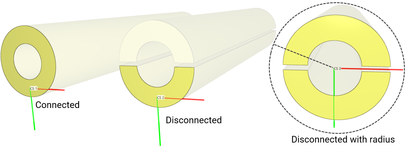
Each pipe is associated with an output section defined with a coordinate system.
- The output section for the first pipe should give the full section area.
- The output section for the second pipe should only give half the section area since the pipe is disconnected.
- The output section for the third pipe should give the full section area since the parameter section radius, $R$ is defined in the command.
CALCULATIONS:
Section area full pipe = $(\pi \cdot {r_{outer}}^{2})-(\pi \cdot {r_{inner}}^{2}) = (\pi \cdot 0.1^2)-(\pi \cdot 0.05^2) = 0.02356 \ m^2$
Section area half pipe = $\frac{(\pi \cdot {r_{outer}}^{2})-(\pi \cdot {r_{inner}}^{2})}{2}= 0.01178 \ m^2$
Targets:
- $Section \ area \ pipe \ 1 = 0.02356 \ m^2$
- $Section \ area \ pipe \ 2 = 0.01178 \ m^2$
- $Section \ area \ pipe \ 3 = 0.02356 \ m^2$
Tests
This benchmark is associated with 1 tests.
Simply supported beam central load
"Optional title"
coid, entype, enid, csysid, $R$
Tested parameters: coid, entype, enid, csysid.
This model tests the functionality of the command *OUTPUT_SECTION. The test model is a simply supported beam of length $1 \ m$, width & height $0.05 \ m$ subjected to a central load of $1000 \ N$. Both ends of the beam are restricted in Y & Z-direction. See Figure 1.
From Euler-Bernoulli beam theory, the maximum deflection and moments can be caluclated. The maximum deflection at mid section is:
$$ \delta_{max} = \frac{PL^3}{48EI} $$
And moment along the beam length is:
$$ M(x) = \frac{Px}{2} \ , \ for \ 0 \leq x \leq \frac{L}{2} $$
$$ M(x) = \frac{P(L-x)}{2} \ , \ for \ \frac{L}{2} < x\leq L $$
Output sections are placed at $x= \frac{L}{4}$, $x= \frac{L}{2}$ & $x= \frac{3L}{4}$ to extract bending moments and an output sensor is placed at the mid section to extract maximum deflection of the beam.
The maximum displacement at mid section vs. time from the simulation is plotted with an analytical function obtained from Euler-Bernoulli beam theory. See Figure 2.
The bending moment vs. time from the simulation at output section $x= \frac{L}{4}$ & $x= \frac{3L}{4}$ is plotted with an analytical function obtained from Euler-Bernoulli beam theory. See Figure 3.
The bending moment vs. time from the simulation at output section $x= \frac{L}{2}$ (mid section) is plotted with an analytical function obtained from Euler-Bernoulli beam theory. See Figure 4.
Targets:
- Mid section, maximum deflection = $-0.0002 \ m$
- Output section $x= \frac{L}{4}$, maximum resultant moment = $125 \ Nm$
- Output section $x= \frac{3L}{4}$, maximum resultant moment = $125 \ Nm$
- Output section $x= \frac{L}{2}$, maximum resultant moment = $250 \ Nm$
- All output sections, section area = $0.0025 \ m^2$.
Tests
This benchmark is associated with 1 tests.
*OUTPUT_SENSOR
Sensor output
"Optional title"
coid, pid, $x_0$, $y_0$, $z_0$, $R$, csysid, ref, lagrange
This tests the *OUTPUT_SENSOR command. The benchmark consists of four tests:
The first tests the position/velocity/acceleration outputs from the command. Two sensors are placed on the moving body. One sensor outputs values in a local coordinate system that follows the moving body. This sensor should only report zero values. The test is carried out using the model described in the *OUTPUT_NODE benchmark. Refer to this for figures and calculations.
The second test checks the pressure/stress/strain outputs from the command. A cubic element is stretched using *BC_MOTION to produce the values of interest.
The third test checks the damage output from the command. A cube of eight linear elements is pulled apart using *BC_MOTION to produce the values of interest. The output should report a damage of about $0.22$.
The fourth test checks the Discrete Particle (DP) outputs from the command. A simple blast model with air-, soil- and high explosive discrete particles is run with two sensors. One sensor is located within the soil domain above the charge, the other right above the sand in the air domain. Number of particles in the sensors are checked for version control.
All together, the following outputs are checked:
| X-coordinate | Y-coordinate | Z-coordinate |
| X-displacement | Y-displacement | Z-displacement |
| X-velocity | Y-velocity | Z-velocity |
| Stress XX | Stress YY | Stress ZZ |
| Stress XY | Stress YZ | Stress ZX |
| Effective stress | Pressure | Effective plastic strain |
| Volumetric strain | Max principal surface strain | Min principal surface strain |
| Damage | Air density (DP) | Soil density (DP) |
| Number of particles (DP) |
Tests
This benchmark is associated with 4 tests.
*OUTPUT_SENSOR_THICKNESS
Components with varying thickness
"Optional title"
coid, pid, $x_0$, $y_0$, $z_0$, fixed, $t_{beg}$, $t_{end}$
$n_x$, $n_y$, $n_z$
Tested parameters: coid, pid, $x_0$, $y_0$, $z_0$, fixed, $n_x$, $n_y$, $n_z$.
This model tests the command *OUTPUT_SENSOR_THICKNESS. The test consists of three components with varying thickness, an irregular box, a cylinder and a pipe. Thickness sensors are positioned at one end of the components, fixed in space. The components translates in the horizontal plane, going from minimum to maximum thickness relative to the thickness sensors which measures the increasing thickness. See Figure 1.
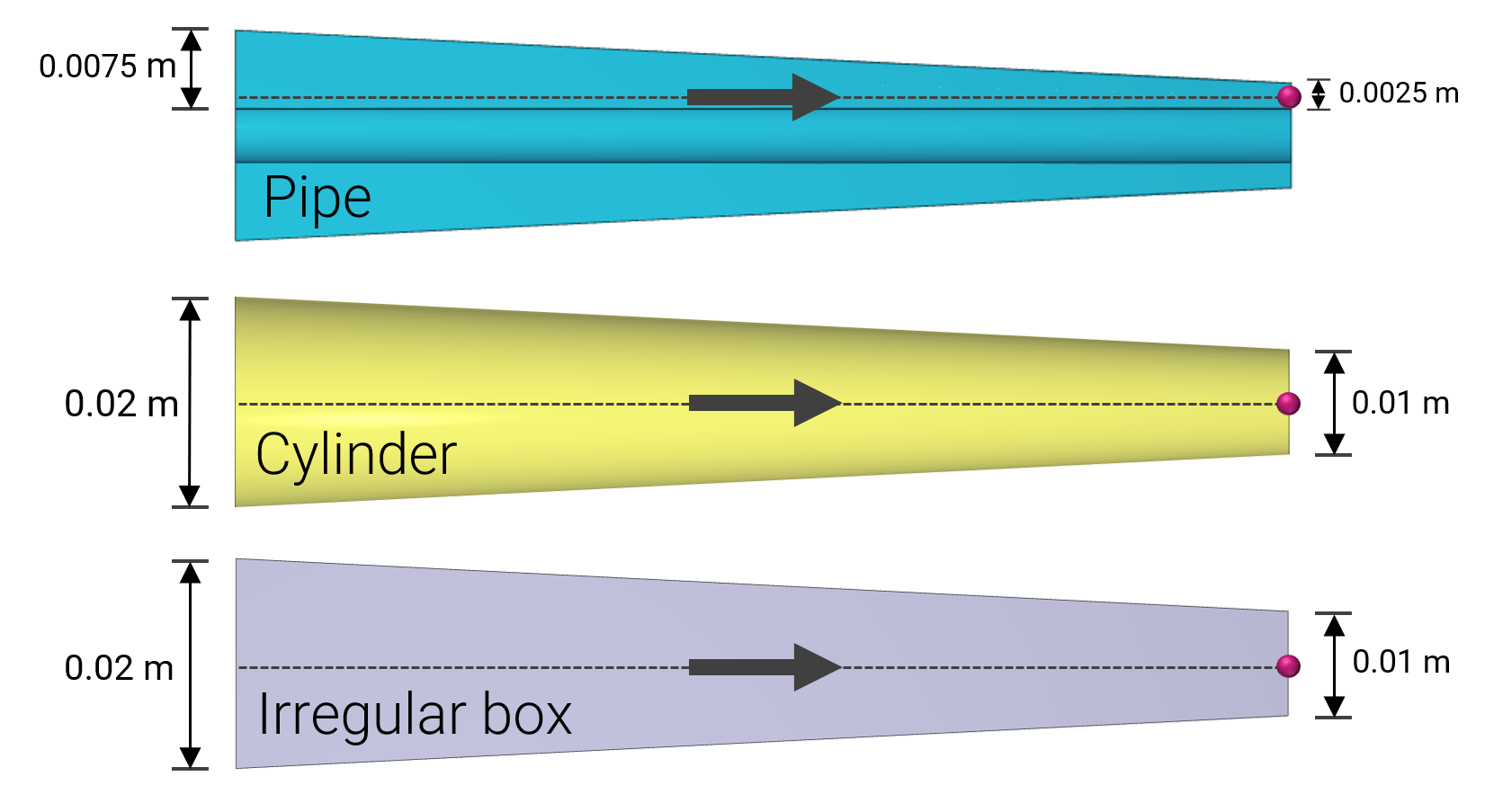
The thickness of the components measured by the thickness sensors can be seen in Figure 2.
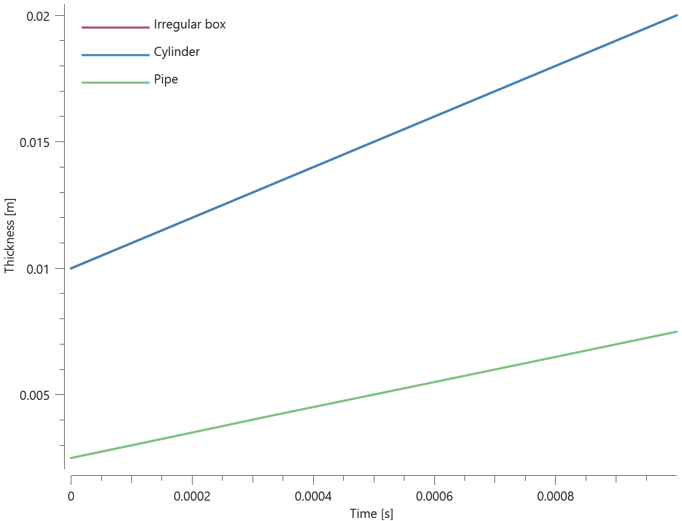
First and final thickness is checked for version control.
Tests
This benchmark is associated with 1 tests.
Control rolling process with thickness sensor
"Optional title"
coid, pid, $x_0$, $y_0$, $z_0$, fixed, $t_{beg}$, $t_{end}$
$n_x$, $n_y$, $n_z$
Tested parameters: coid, pid, $x_0$, $y_0$, $z_0$, fixed, $n_x$, $n_y$, $n_z$.
This model tests the command *OUTPUT_SENSOR_THICKNESS in a simple rolling process. A thickness sensor is used to adjust the vertical position of the rolls. This is done with a python script which controls the vertical velocity of the rolls by subtracting measured thickness with target thickness.
$$ v_{vertical} = t_{measured} - t_{target} $$
Where $t_{measured}$ is the current thickness measured from the thickness sensor and $t_{target}$ is a predetermined target thickness of the workpiece. The workpiece moves forward in the positive X-direction and and when it reaches the sensor, the rolls are instructed to begin moving vertically.
See Figure 1.
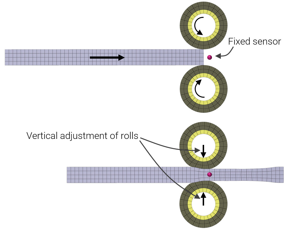
The resulting thickness from the rolling process is converging towards the target thickness of $0.06 \ m$, see Figure 2.
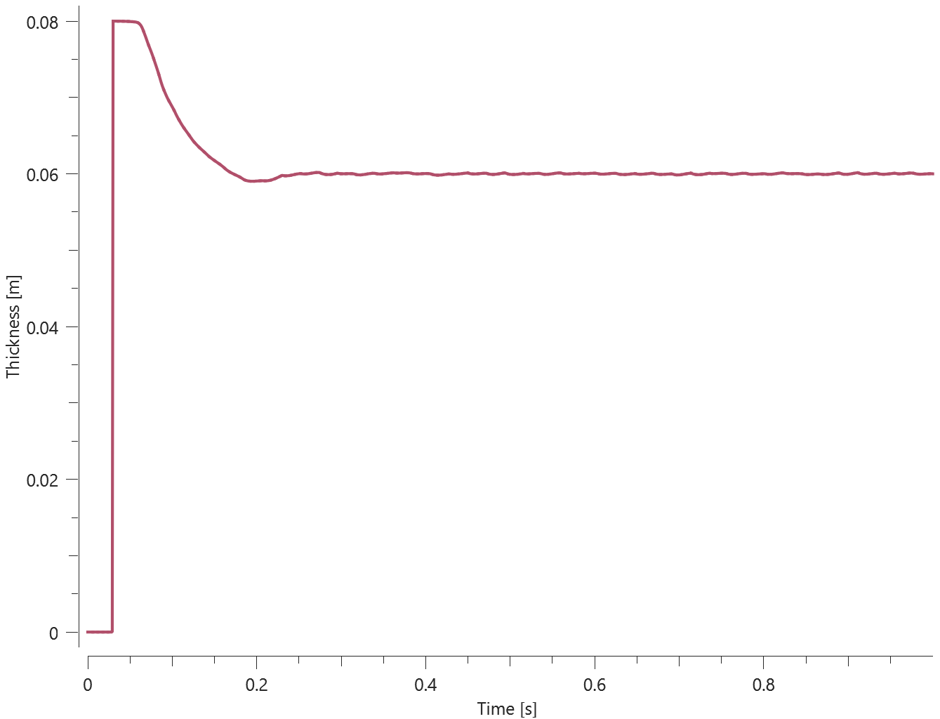
Thickness is checked for version control.
Tests
This benchmark is associated with 1 tests.
*OUTPUT_USER_COLLECTION
Deforming metal ring
"file_name"
coid, outint, outform
entype, enid, dptype, fid, extensive
Tested parameters: file_name, coid, outint, outform, entype, enid, dptype, fid, extensive.
The model tests the functionality of the command *OUTPUT_USER_COLLECTION. The test consists of a dynamically deforming metal ring. The internal energy (extensive variable) is collected for each element with *OUTPUT_USER_COLLECTION.
The test setup is displayed in Figure 1.
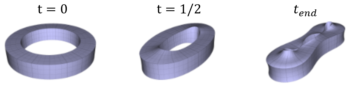
The total internal energy is summed up for each element and compared with the internal energy output of the entire model from energy.out. See Figure 2.

Tests
This benchmark is associated with 1 tests.
Revolving bar
"file_name"
coid, outint, outform
entype, enid, dptype, fid, extensive
Tested parameters: file_name, coid, outint, outform, entype, enid, dptype, fid.
The model tests basic functionality of the command *OUTPUT_USER_COLLECTION. A 2D bar with length $1 \ m$ is revolving 1 lap around its Z-axis during 1 second. It is fixed in one end. The bar is divided into 10 elements. *OUTPUT_USER_COLLECTION is used to collect velocity history of the elements of the bar.
The test setup is displayed in Figure 1.
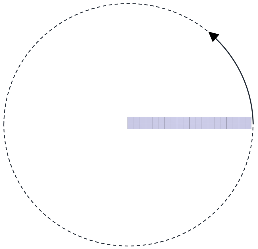
An output sensor is placed in the middle of the element furthest out of the bar ($0.95 \ m$), measuring velocity for comparison with the elements collected. The velocity will be highest the furthest out of the bar: $v = w = 2\pi \ m/s$
Targets:
- Maximum sensor x- and y-velocity from output sensor: $0.95 \cdot 2\pi = 5.9690 \ m/s$
- Maximum velocity element 10 from .out-file: $5.9690 \ m/s$
Tests
This benchmark is associated with 1 tests.
*PARAMETER
Defined and redefined parameters
%param = expression, "description", rid, quantity
This tests the *PARAMETER command. Four elements are set in motion by four *BC_MOTION commands. Motions are defined by a sine function of the time.
$$ f=sin(amp*360{t}/{t_{end}}) $$
Between each *BC_MOTION command, the amplitude ($amp$) is redefined by a new *PARAMETER command. The maximum displacement of the four elements should therefore all differ and this is checked for version control. See Figure 1.
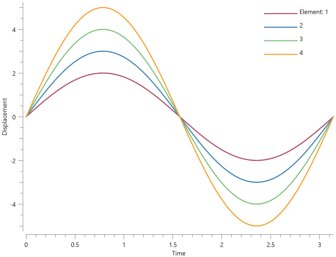
Tests
This benchmark is associated with 1 tests.
*PARAMETER_DEFAULT
Parameter order
"Optional title"
%param = expression, "description", rid, quantity
Tested parameters: param = expression, description
This model tests that parameters defined within the command *PARAMETER_DEFAULT are overwritten correctly when also defined within the command *PARAMETER.
The test setup consists of two spheres that are in free fall due to gravity. In total, the parameter gravity is defined four times in the following order:
*PARAMETER
gravity = 0.1, "random value (this value should be overwritten)"
*PARAMETER
gravity = 1.62, "gravity on moon"
*PARAMETER_DEFAULT
gravity = 9.81, "gravity on earth (This value should be overwritten)"
#Here first sphere is assigned gravity
*PARAMETER
gravity = 9.76, "gravity at equator"
#Here second sphere is assigned gravity
Targets:
- Sphere 1. Acceleration in Z-direction = -1.62 m/s
- Sphere 2. Acceleration in Z-direction = -9.76 m/s
Tests
This benchmark is associated with 1 tests.
*PART
Element erosion
"Optional title"
pid, mid, eosid, $h$, $\alpha_{max}$, $\Delta t^{erode}$, $\varepsilon_{geo}^{erode}$, $\varepsilon_v^{erode}$, $N_{perode}$, $R_{perode}$, $\Delta t_{perode}$
The element erosion options in *PART are verified in this test.
Tested parameters: $\Delta t^{erode}$, $\varepsilon_{geo}^{erode}$ and $\varepsilon_v^{erode}$.
Three pair of cubes are defined. Each pair are used to verify a certain erosion option.
The first pair is used to verify element erosion due to small time step size. Both cubes are volumetricially compressed, causing the time step to drop as the simulation progress. The final time step size in the simulation is denoted as $\Delta t_{final}$.
The time step size below which elements are eroded is defined as $\Delta t ^{erode} = 0.99 \cdot \Delta t_{final}$ for one of the cubes and as $\Delta t ^{erode} = 1.01 \cdot \Delta t_{final}$ for the other.
The second pair is used to verify element erosion due to large effective deviatoric geometric strain. Both cubes are subjected to a shear deformation and the final effective deviatoric geometric strain is defined as $\varepsilon_{geo,final}$.
The effective deviatoric geometric strain above which elements are eroded is defined as $\varepsilon_{geo}^{erode} = 0.99 \cdot \varepsilon_{geo,final}$ for one of the cubes and as $\varepsilon_{geo}^{erode} = 1.01 \cdot \varepsilon_{geo,final}$ for the other. The final effective deviatoric geometric strain for the defined deformation is verfied in a seperate script.
The third pair is used to verify element erosion due to large volumetric strain. Both cubes are volumetrically expanded, and the final volumetric strain is defined as $\varepsilon_{v,final}$.
The volumetric strain above which elements are eroded is defined as $\varepsilon_v^{erode} = 0.99 \cdot \varepsilon_{v,final}$ for one of the cubes and as $\varepsilon_v^{erode} = 1.01 \cdot \varepsilon_{v,final}$ for the other. The final volumetric strain for the defined deformation is verified in a separate script.
At termination, one of the cubes in each pair should have been eroded.
Tests
This benchmark is associated with 1 tests.
Smoothing
"Optional title"
pid, mid, eosid, $h$, $\alpha_{max}$, $\Delta t^{erode}$, $\varepsilon_{geo}^{erode}$, $\varepsilon_v^{erode}$, $N_{perode}$, $R_{perode}$, $\Delta t_{perode}$
This tests the $\alpha_{max}$ (external element face smoothing angle) feature of the *PART command. The set-up is two cylinders of slightly different mesh density. The face of the first cylider is an eight angled polygon 45°, the face of the second is a twelve angled polygon 30°. Both parts are given an input of a max smoothing 40°, so only the second cylinder should be smoothened. All elements are cubic. Coordinates are checked for version control. See Figure 1.
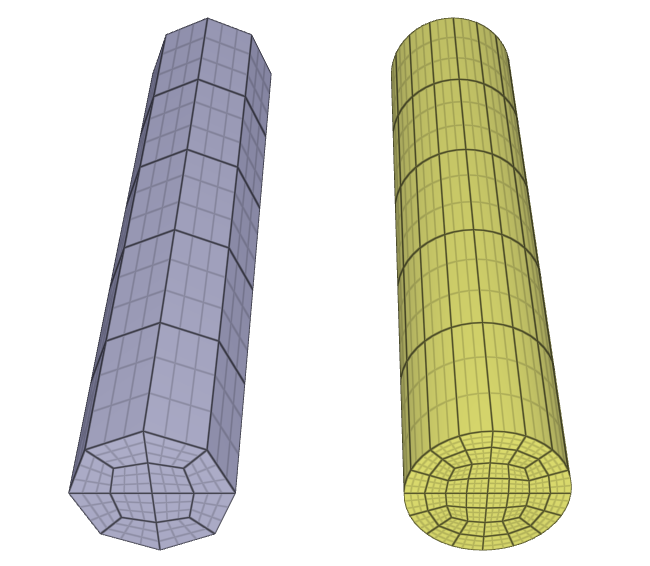
Tests
This benchmark is associated with 1 tests.
*PARTICLE_DETONATION
Detonation geometry ID
"Optional title"
dpid
$x_d$, $y_d$, $z_d$, $t_d$, $R$, fast, gid, sid
Tested parameters: dpid, $x_d$, $y_d$, $z_d$, $t_d$, gid.
This model tests the parameter $gid$ in *PARTICLE_DETONATION, which is used to specify a detonation geometry ID. The detonation point will be neglected and all particles inside the geometry will be initiated at time $t_d$.
The test consists of two spherical discrete particle HE subdomains. A detonation point is set to one of the geometry, however, the detonation geometry ID is specified to the other geometry. The detonation process is thus limited to the subdomain specified by the detonation geometry ID.
It is tested that only the subdomain specified by the detonation geometry ID is detonated. Further, sensors are deployed to ensure that all particles inside the geometry will be initiated at time $t_d$.
The test setup can be seen in Figure 1.
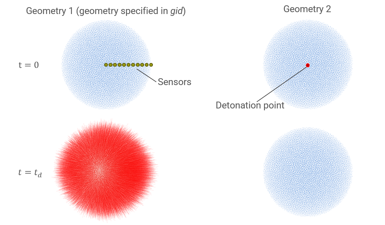
Chemical energy vs. time can be seen in Figure 2.
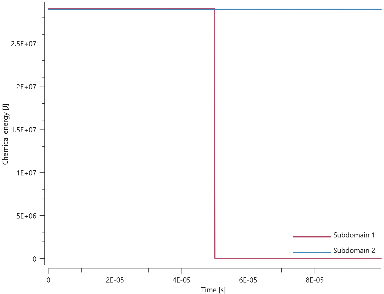
Detonation is set to $t = t_d / 2$. The time the detonation front arrives at the sensors can be seen in Figure 3.
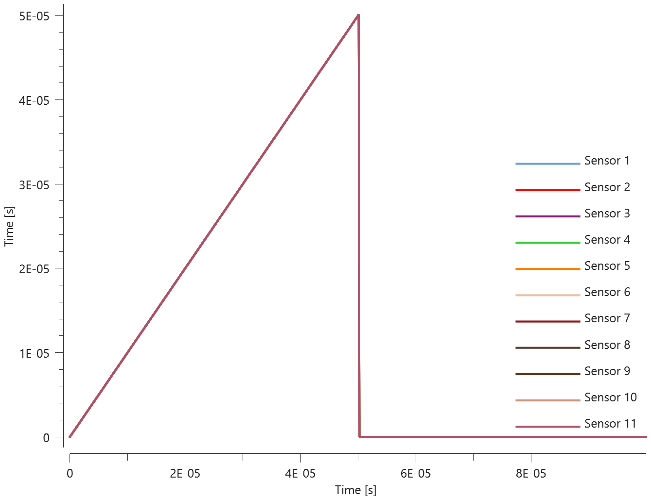
First and last value of chemical energy and the time the detonation front arrives at the sensors is checked for version control.
Tests
This benchmark is associated with 1 tests.
Detonation radius
"Optional title"
dpid
$x_d$, $y_d$, $z_d$, $t_d$, $R$, fast, gid, sid
Tested parameters: dpid, $x_d$, $y_d$, $z_d$, $t_d$, $R$.
This model tests the parameter $R$ in *PARTICLE_DETONATION, which is used to limit the distance the detonation front is allowed to propagate through programmed burn. The test consists of two spherical discrete particle HE subdomains both with an inner radius of $10 \ mm$ and outer radius of $20 \ mm$. A detonation point is set in the centre of each sphere. One of the subdomain's detonation radius is limited to its inner radius by setting $R = 0.01$. It is tested that only the subdomain without the radius limitation is triggered from the detonation.
The test setup can be seen in Figure 1.
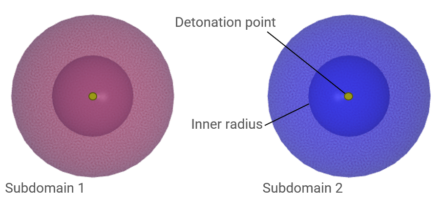
Chemical energy vs. time can be seen in Figure 2.

First and last value of chemical energy is checked for version control.
Tests
This benchmark is associated with 1 tests.
Radial detonation path
"Optional title"
dpid
$x_d$, $y_d$, $z_d$, $t_d$, $R$, fast, gid, sid
Tested parameters: dpid, $x_d$, $y_d$, $z_d$, $t_d$, fast.
This model tests the parameter $fast$ in *PARTICLE_DETONATION. By default the detonation front propagates from particle to particle. Setting $fast=1$ assumes a simple radial detonation front instead. The test consists of two torus shaped discrete particle HE subdomains with detonation points set to one of the sides. Sensors are placed on the other sides to measure the arrival of the detonation front. See Figure 1.
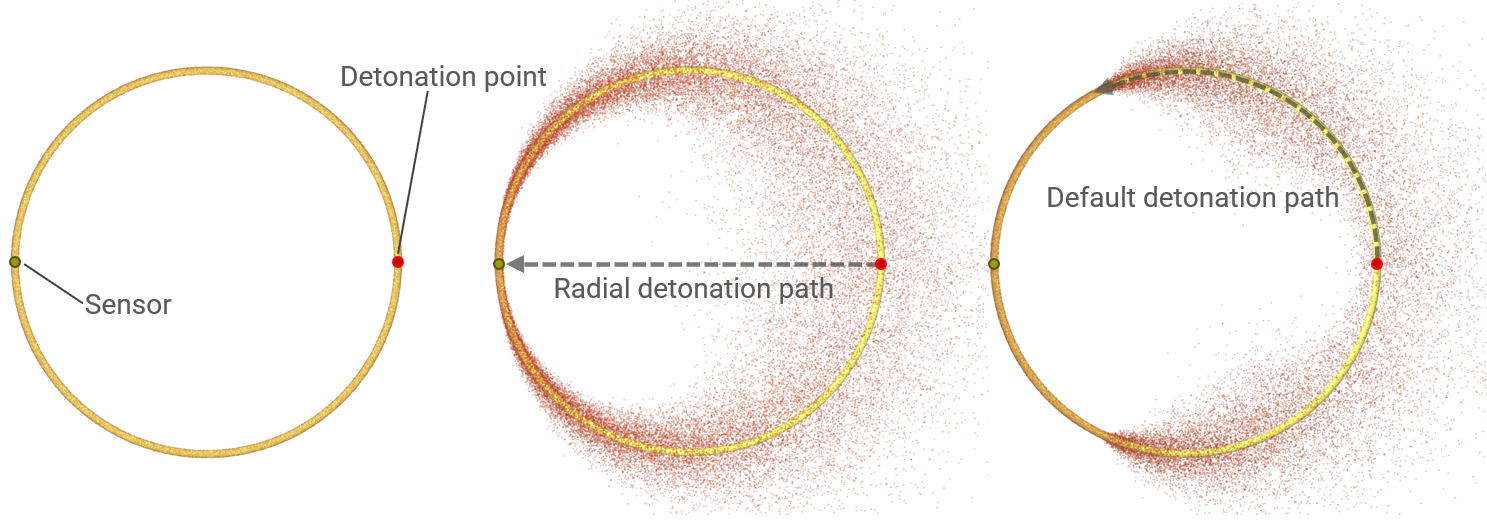
The detonation time at the sensor should be:
$$ t_{d_S} = t_{d}+\frac{r}{D} $$
Where $t_{d}$ is the detonation time at the detonation point (set to zero), $r$ is the distance from the detonation point and $D$ is the detonation velocity.
Subdomain 1, Radial detonation path:
$$ t_{d_{S1}} = t_{d}+\frac{r}{D}=0+\frac{0.1}{6930}= 1.443 \cdot 10^{-5} $$
Subdomain 2, Default detonation path:
$$ t_{d_{S2}} = t_{d}+\frac{r}{D}=0+\frac{(\pi \cdot 0.1)/2}{6930}= 2.266 \cdot 10^{-5} $$
The detonation time at the sensors is checked for version control.
Tests
This benchmark is associated with 1 tests.
Subdomain limit
"Optional title"
dpid
$x_d$, $y_d$, $z_d$, $t_d$, $R$, fast, gid, sid
Tested parameters: dpid, $x_d$, $y_d$, $z_d$, $t_d$, sid.
This model tests the parameter $sid$ in *PARTICLE_DETONATION, which is used to limit the detonation process to one specific subdomain. The test consists of two spherical discrete particle HE subdomains on either side of a detonation point. The detonation point is limited to one of the subdomains with the parameter $sid$. It is tested that only one of the subdomains is triggered from the detonation. The test setup can be seen in Figure 1.
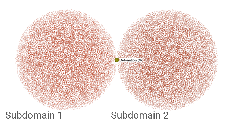
Chemical energy vs. time can be seen in Figure 2.
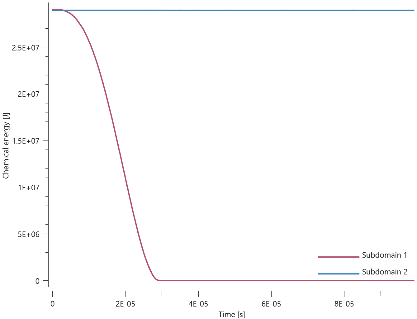
First and last value of chemical energy is checked for version control.
Tests
This benchmark is associated with 1 tests.
*PARTICLE_DOMAIN
Binomial distribution
entype, enid, N${}_p$, $\mu$, $pfac$, $c_{dec}$, xsmooth, $t_{end}$
$x_0$, $y_0$, $z_0$, $x_1$, $y_1$, $z_1$
bc${}_{x0}$, bc${}_{y0}$, bc${}_{z0}$, bc${}_{x1}$, bc${}_{y1}$, bc${}_{z1}$
$\delta_0^{max}$, ctype, SPH${}_{uniform}$
This model tests particle-structure contact and probability distribution of discrete particles. The test setup is a model of a Galton board, which can be used to demonstrate central limit theorem. 50,000 soil particles with similar properties to sand are moving down the Galton board. The particles will either go to the left or right as they come in contact with the pegs. The state at beginning, middle and end of the simulation is shown in Figure 1.
The simulation indicates that with a sufficient sample size, the binomial distribution approximates a normal distribution from the random motion of the discrete particles. The number of particles that end up in each column is summed in Figure 2.
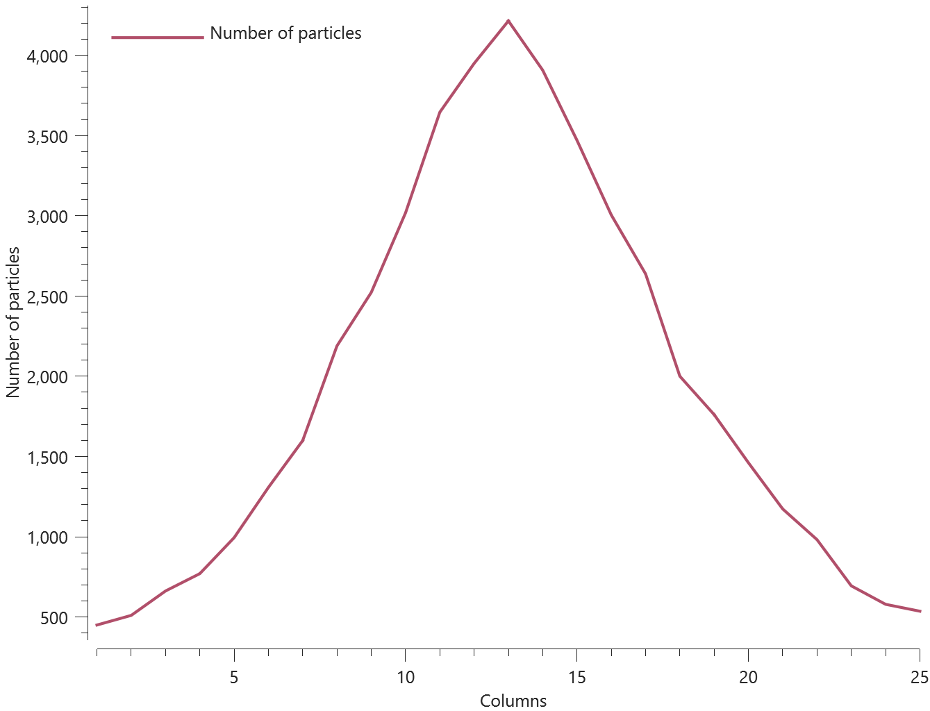
Maximum number of particles in each column is checked for version control.
Tests
This benchmark is associated with 1 tests.
Convergence test
entype, enid, N${}_p$, $\mu$, $pfac$, $c_{dec}$, xsmooth, $t_{end}$
$x_0$, $y_0$, $z_0$, $x_1$, $y_1$, $z_1$
bc${}_{x0}$, bc${}_{y0}$, bc${}_{z0}$, bc${}_{x1}$, bc${}_{y1}$, bc${}_{z1}$
$\delta_0^{max}$, ctype, SPH${}_{uniform}$
The commands *PARTICLE_HE and *PARTICLE_SOIL are also used in this test.
A high-explosive charge is buried and detonated in sand. A rigid plate is located a distance from the sand domain as seen in Figure 1. The model is run with both presets of sand (dry and wet) and the number of particles investigated are: 50k, 100k, 200k, 400k and 800k.
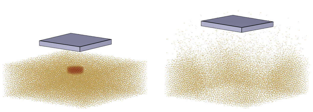
The impulse transfer from the high-explosive and sand to the plate is presented in Figure 2 (dry sand) and Figure 3 (wet sand). The impulse transfer is checked for version control.
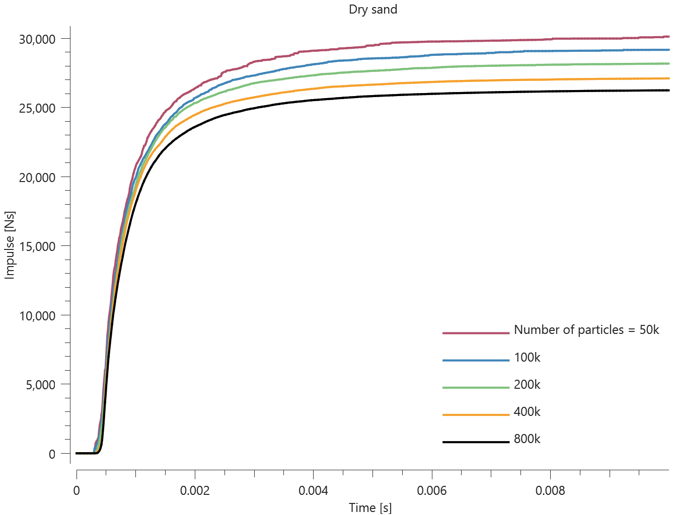
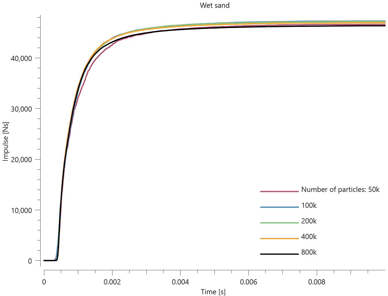
Tests
This benchmark is associated with 10 tests.
*PARTICLE_DOMAIN_CLEANUP
Deactivate particles
"Optional title"
sid, $t_{clean}$, gid, repeat, $m_{min}$, $W_{min}$, $v_{min}$
$n_x$, $n_y$, $n_z$
Tested parameters: sid, $t_{clean}$, gid
This model tests the *PARTICLE_DOMAIN_CLEANUP command. A number of subdomains of particles are created with iterative control. Inside the repeat loop, 16 spheres are being defined. The spheres are filled with particles and the command *PARTICLE_DOMAIN_CLEANUP is used to deactivate all the particles.
The test setup is displayed in Figure 1.
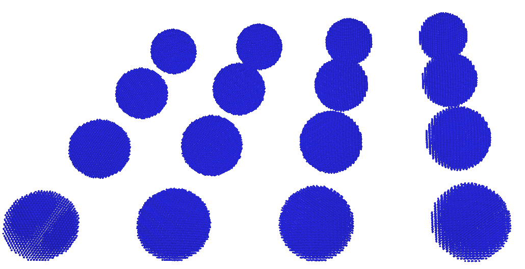
There should be no particles left at end of simulation.
Tests
This benchmark is associated with 1 tests.
repeat parameter
"Optional title"
sid, $t_{clean}$, gid, repeat, $m_{min}$, $W_{min}$, $v_{min}$
$n_x$, $n_y$, $n_z$
Tested parameters: sid, $t_{clean}$, gid, repeat
This model tests the parameter repeat in the command *PARTICLE_DOMAIN_CLEANUP. Four spheres of particles are equally distanced apart. The spheres are travelling in the X-direction with a constant velocity towards a geometry in space that will cover only the upper half of the spheres. See Figure 1.
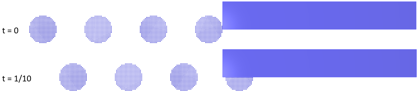
The command *PARTICLE_DOMAIN_CLEANUP is used to de-activate all particles that are within this geometry at a certain time. The cleanup time is defined as 1/10 of the total simulation time. However, because repeat is activated, the de-activation of particles will occur in the interval of 1/10 of the simulation time, i.e. 10 times in total.
Only half of the particles should remain at end of simulation.
Tests
This benchmark is associated with 1 tests.
*PARTICLE_HE
Static overpressure
"Optional title"
sid, overlay
type, gid, follow, $dsf$, ., ., ., $t_{end}$
$\rho_0$, $e_0$, $\gamma$, $v$, $D$
This model tests the static gas pressure at thermal equilibrium for all callibrated high-explosives with the command *PARTICLE_HE. A high-explosive charge is detonated within a rigid spherical container, see Figure 1.
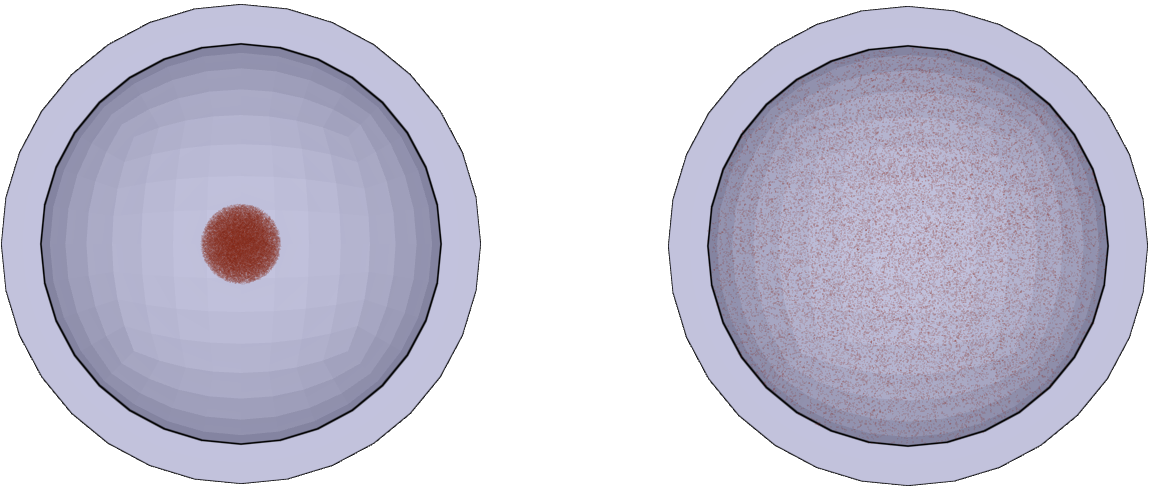
The final static overpressure inside the sphere is checked against calculations based on the ideal gas law. The test configurations and paramater values can be seen in Table 1.
| Abbreviation | Explaination |
|---|---|
| $r_c$ | - Container radius |
| $r_{he}$ | - HE charge radius |
| $e_{he}$ | - HE energy density |
| $e$ | - Energy density at equllibrium |
| $\gamma$ | - Fraction between $C_p$ and $C_v$ at zero co-volume (ideal gas regime) |
| $p$ | - Static pressure (ideal gas law) |
| $p'$ | - Overpressure |
| Explosive | $r_c \ [m]$ | $r_{he} \ [m]$ | $e_{he} \ [GJ/m^3]$ | $e=e_{he} \cdot (r_{he}/r_c)^3 \ [MJ/m^3]$ | $\gamma \ [-]$ | $p=(\gamma-1) \cdot e \ [MPa]$ | $p'=p-1 \ bar \ [MPa]$ |
|---|---|---|---|---|---|---|---|
| ANFO | 0.5 | 0.1 | 2.9 | 23.2 | 1.280 | 6.496 | 6.396 |
| C4 | 0.5 | 0.1 | 9.0 | 72.0 | 1.270 | 19.44 | 19.34 |
| COMP. A-3 | 0.5 | 0.1 | 8.9 | 71.2 | 1.442 | 31.47 | 31.37 |
| COMP. B (grade A) | 0.5 | 0.1 | 8.5 | 68.0 | 1.428 | 29.104 | 29.004 |
| HMX | 0.5 | 0.1 | 10.5 | 84.0 | 1.345 | 28.980 | 28.880 |
| LX-10-1 | 0.5 | 0.1 | 10.4 | 83.2 | 1.606 | 50.4192 | 50.3192 |
| LX-14-0 | 0.5 | 0.1 | 10.2 | 81.6 | 1.576 | 47.0016 | 46.9016 |
| MCX-6100 | 0.5 | 0.1 | 7.6 | 60.8 | 1.404 | 24.563 | 24.463 |
| NSP-711, m/46 | 0.5 | 0.1 | 7.05 | 56.4 | 1.315 | 17.766 | 17.666 |
| OCTOL 78-22 | 0.5 | 0.1 | 9.6 | 76.8 | 1.598 | 45.926 | 45.826 |
| PBXN-110 | 0.5 | 0.1 | 8.7 | 69.6 | 1.375 | 26.100 | 26.000 |
| PBXN-9010 | 0.5 | 0.1 | 9.0 | 72.0 | 1.451 | 32.472 | 32.372 |
| PETN | 0.5 | 0.1 | 10.1 | 80.8 | 1.621 | 50.177 | 50.077 |
| TETRYL | 0.5 | 0.1 | 8.2 | 65.6 | 1.442 | 28.995 | 28.895 |
| TNT | 0.5 | 0.1 | 7.0 | 56.0 | 1.299 | 16.744 | 16.644 |
Tests
This benchmark is associated with 16 tests.
*PARTICLE_SOIL
Sand slug impact
"Optional title"
sid
type, gid, $dsf$, ., ., ., ., $t_{end}$
$\rho_0$, $k$, $\mu$, $\xi$, $v$, $\eta$
This model tests the command *PARTICLE_SOIL
A sand slug impacts a rigid wall at a velocity of $v = 500 \ m/s$. See Figure 1. The transferred impulse should be close to $m\cdot v$, where $m$ is the total mass of the sand. Both predefined sand types (dry and wet) are tested. See Table 1.
| Sand properties | Volume, $V \ [m^3]$ | Density, $\rho \ [kg/m^3]$ | Mass, $m=V \cdot \rho \ [kg]$ | Momentum, $I=m\cdot v \ [Ns]$ | Kinetic energy, $Wk=0.5 \cdot m \cdot v^2 \ [MJ]$ |
|---|---|---|---|---|---|
| Dry sand | 8.0e-3 | 1620 | 12.96 | 6480 | 1.62 |
| Wet sand | 8.0e-3 | 2020 | 16.16 | 8080 | 2.02 |
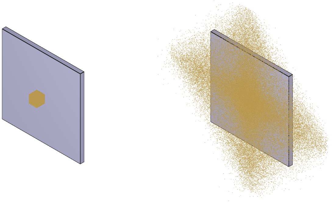
Tests
This benchmark is associated with 2 tests.
*PARTICLE_SPH
Fe to SPH conversion
"Optional title"
sid
mid, gid, correction, $s$, $dsf$, -, slide, $t_{end}$
csysid
This tests the FE to SPH conversion. When elements are eroded they convert to SPH particles. In the test a metal sphere is given an initial velocity and dropped on a metal cube. The test is done twice, once without a errosion criteria for the target cube and once with. With the errosion criteria the cubes element will erode and convert to SPH. The aim of the test is to replicate the result from the test without FE to SPH conversion, hence showing that the method is reliable and does not lose much accuracy.
The sphere is moving in negative Z-direction, therefore the test chekcs the Z-coordinate of the center of the sphere. There is also a check for the total mass of the converted particles and the target cube. One advantage with the convertion is to preserve the mass. Usually when elements are eroded the part will lose mass, when converting to SPH the eroded mass should be contained by the convertion to SPH particles.
Figure 3 shows the final state of the test where the erroded elements have been converted to SPH particles. The FE part is hiddden in the figure.
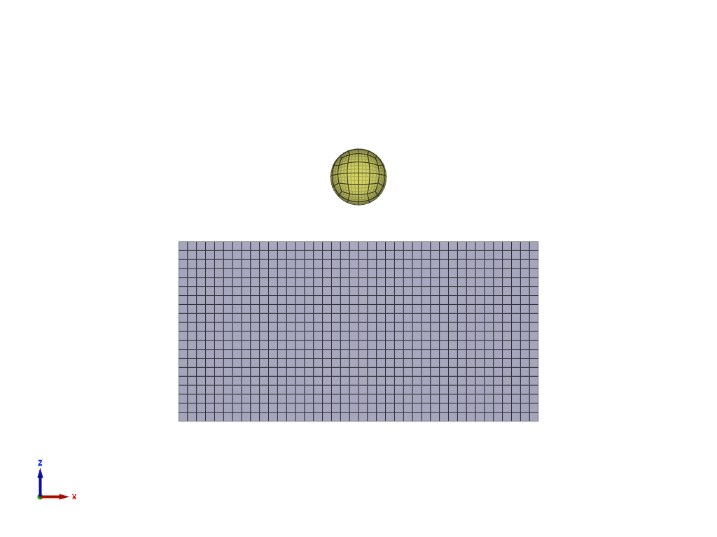
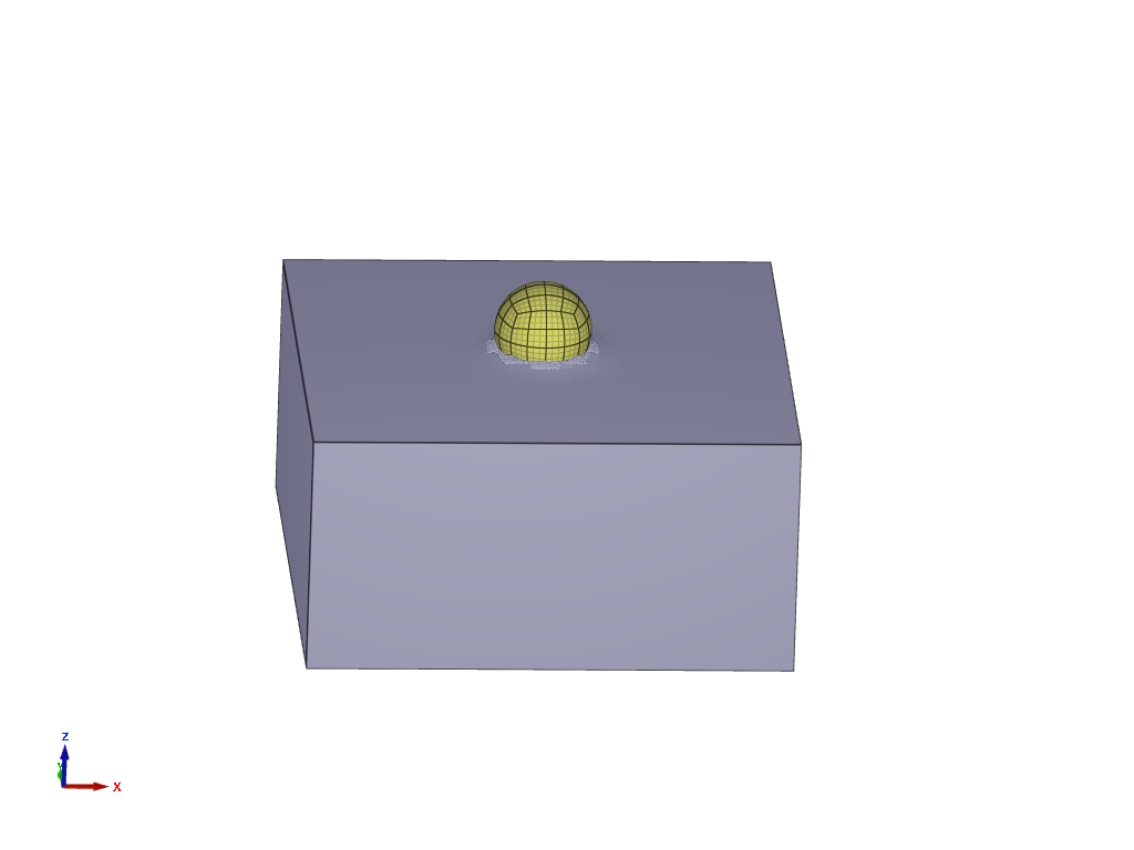
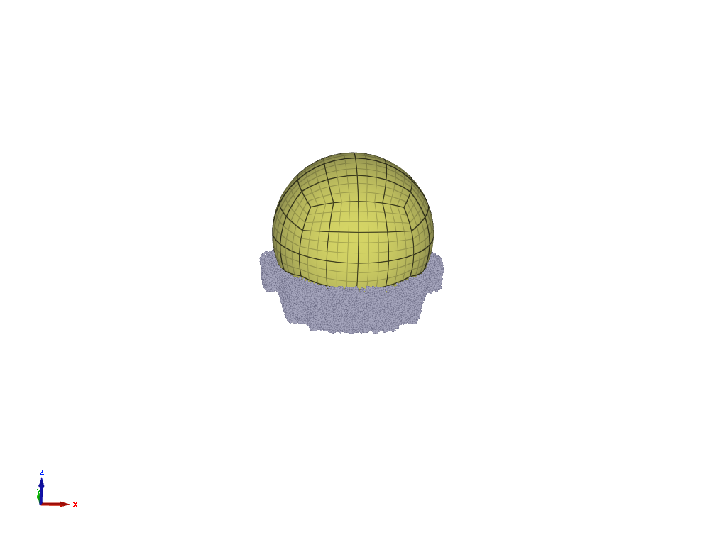
In figure 4 the result from both simulations are compared. Figure 5 shows the mass for the FE part through out the simulation, as well as summed with the SPH particles. Figure 6 shows the total SPH partcile mass during the simulation.
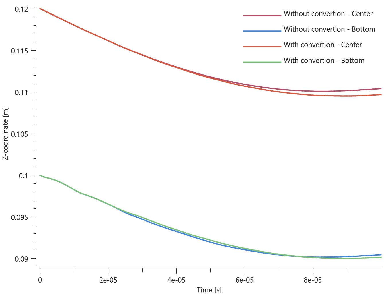
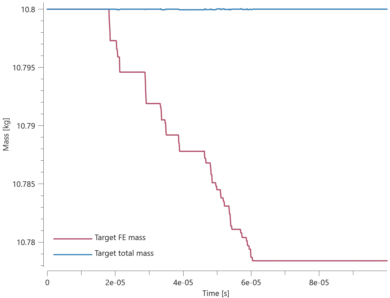
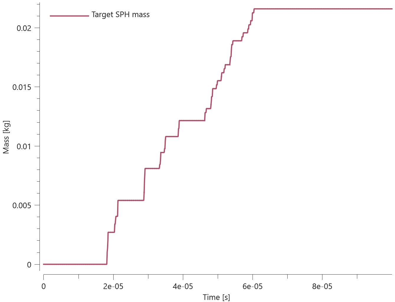
The Z-coordinate at the middle and bottom of the sphere is checked. There is checks for mass of the FE target as well as the SPH target. The energy balance is also checked.
Tests
This benchmark is associated with 1 tests.
Fe to SPH conversion - both parts
"Optional title"
sid
mid, gid, correction, $s$, $dsf$, -, slide, $t_{end}$
csysid
This test is a copy of *PARTICLE_SPH - FE to SPH conversion, but here both FE parts can be converted into SPH particles. This test is also compared to the simulation where no FE parts are converted to SPH particles. The test setup can be found at *PARTICLE_SPH - FE to SPH convertion. Figure 1 shows how parts of the impactor have converted to SPH particles at the final state of the simulation. There is also SPH particles from the target that have been converted from FE showing.
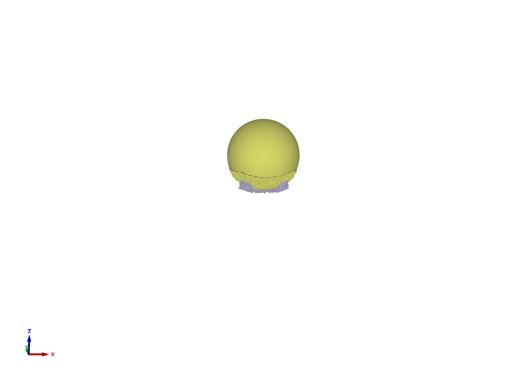
In figure 2 the Z-coordinate in the middle of the impactor is shown and compared to the same sensor from the simulation withouth any convertion. Since the elements in the bottom of the impactor will erode in this test the sensor that was previously placed there is removed.
Figure 3 shows tha mass of the impactor throughout the simulation.
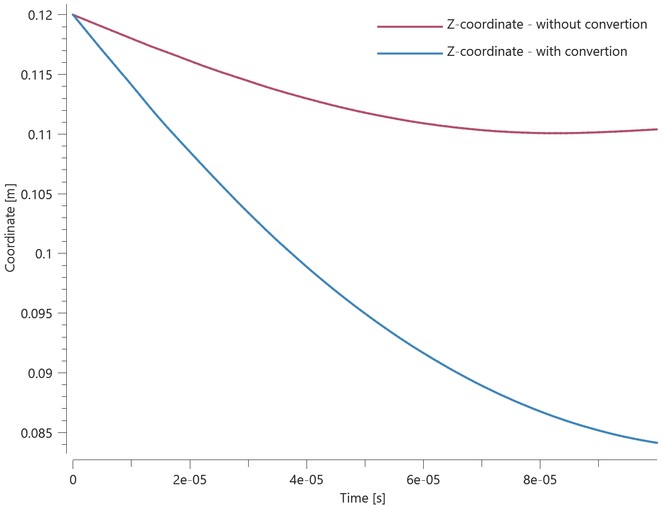
The Z-coordinate at the middle of the sphere is checked. There is checks for mass of both the parts in the simulation, both for FE and SPH. The energy balance is also checked.
Tests
This benchmark is associated with 1 tests.
PARTICLE_SPH - Symmetry
"Optional title"
sid
mid, gid, correction, $s$, $dsf$, -, slide, $t_{end}$
csysid
In this test the symmetry condition when using SPH particles are tested. A taylor bar modelled with SPH particles are subject for impact against a rigid wall. The bar is modelled using quarter symmetry.
Two sensors are placed at the lower part of the model that will deform upon impact. The displacements in x- and y-direction in each sensor are checked for verison control.
*PATH
Impetus module
"Optional title"
pathid
$x_1$, $y_1$, $z_1$
.
$x_{\mathrm{n}}$, $y_{\mathrm{n}}$, $z_{\mathrm{n}}$
Tested parameters: pathid, $x_1$, $y_1$, $z_1$, $x_{\mathrm{n}}$, $y_{\mathrm{n}}$, $z_{\mathrm{n}}$
This model tests the *PATH command. A cube with side length $0.5$ is following a path consisting of four lines of length $1$ and one line of length $\sqrt{2}$. The test setup is displayed in Figure 1.
To instruct the cube to follow this path, the cube is given a prescribed displacement defined by three functions specified in a python script. With the impetus module: "impetus.path", the X-, Y- and Z-coordinates of the path is returned using relative position. The position variable in the module is multiplied by $1.5$, resulting in that the upper limit of the path is exceeded and the return value will be extrapolated from the last path segment.
The sought result is that the cube will travel the total path which is a length of $4+\sqrt{2}$, then continue to travel outside of the path a distance of $\frac{4+\sqrt{2}}{2}$ in the X-direction (same direction as last segment of the path).
To verify that *PATH and the "impetus.path" module is working properly, X-displacement of the cube is checked for first, average and maximum value. This is displayed in Figure 2.
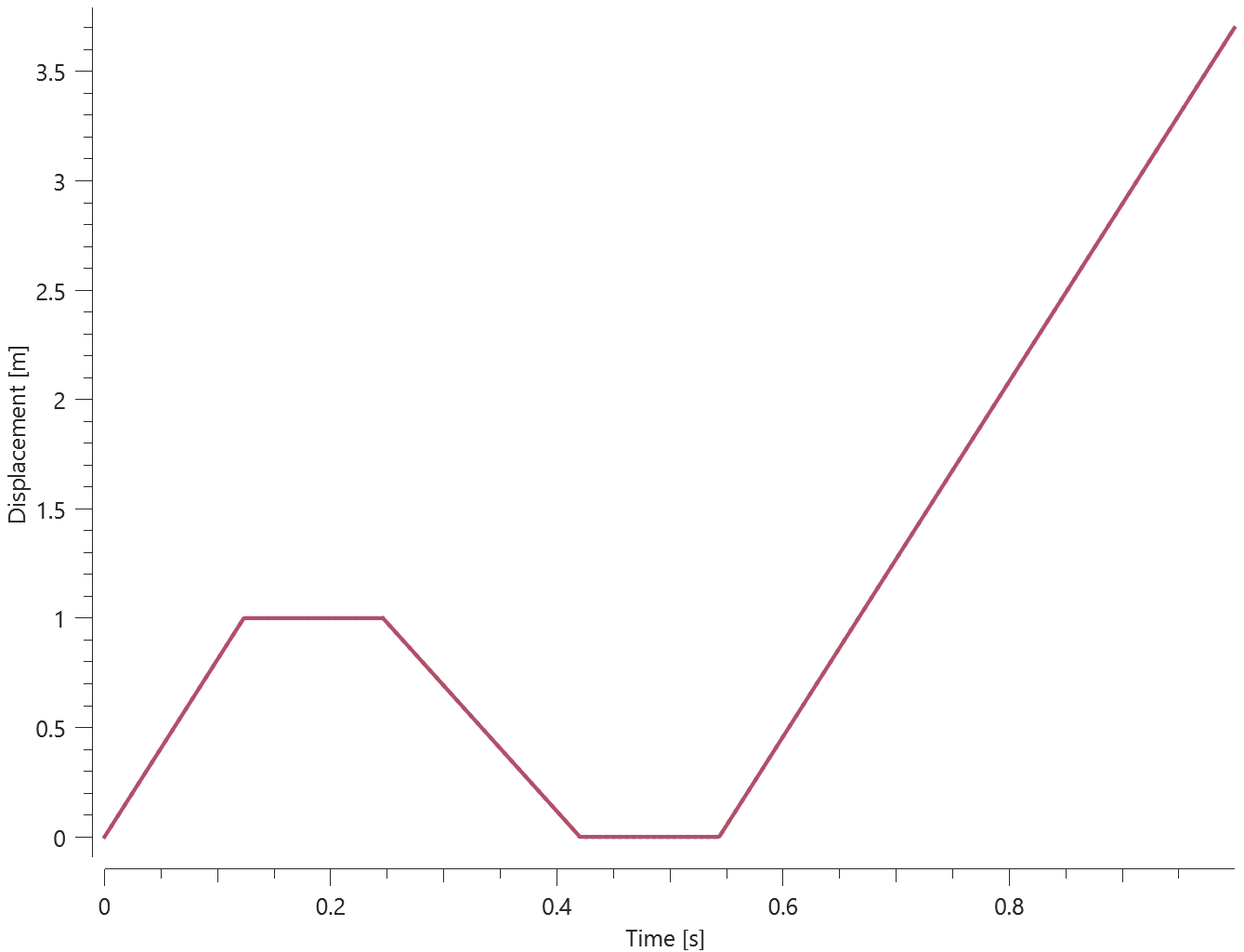
Tests
This benchmark is associated with 1 tests.
*PETRIFY
Bouncing ball with and without petrify
"Optional title"
coid
entype, enid, $t_{on}$, $t_{off}$, multiple
Tested parameters: coid, entype, enid, $t_{on}$, $t_{off}$.
This model tests the *PETRIFY command. A ball is bouncing on a surface. It is then travelling away from the surface to eventually come back for a second bounce. While the ball is in the air in its flight path away from the surface, *PETRIFY is used to temporarily turn the ball into a rigid body. It is then being deactivated when closing in to the surface.
The test setup is displayed in Figure 1.
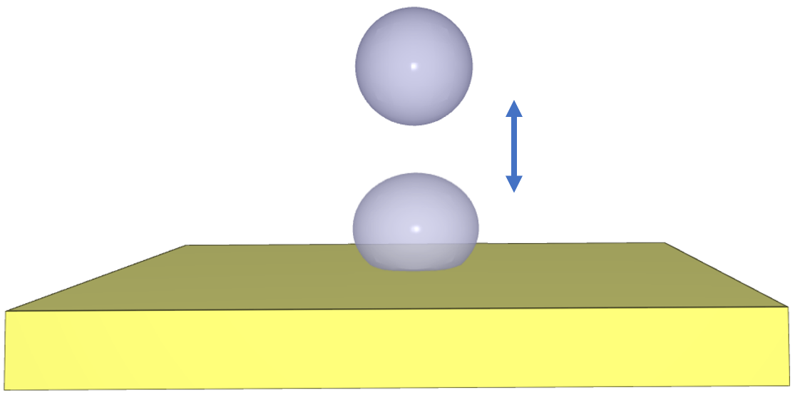
The wanted outcome is that the results should not change significantly with/without *PETRIFY, but the simulation time should be reduced with *PETRIFY.
Targets:
- Number of time steps without petrify = 71192
- Number of time steps with petrify = 22385
- Sensor, sphere. Z-coordinate average value = 0.68215 m
- Sensor, sphere. Z-coordinate last value = 0.43786 m
Result to be within 1% of targets
Tests
This benchmark is associated with 2 tests.
*PRESTRESS_BLIND_HOLE_BOLT
Aligned bolts
pid${}_{bolt}$, pid${}_{plate}$, cid, $sf$, $t_{beg}$, $t_{end}$
Tested parameters: $pid_{bolt}$, $pid_{plate}$, cid.
This model tests the command *PRESTRESS_BLIND_HOLE_BOLT. The test consists of 2 steps. The test setup is displayed in Figure 1.
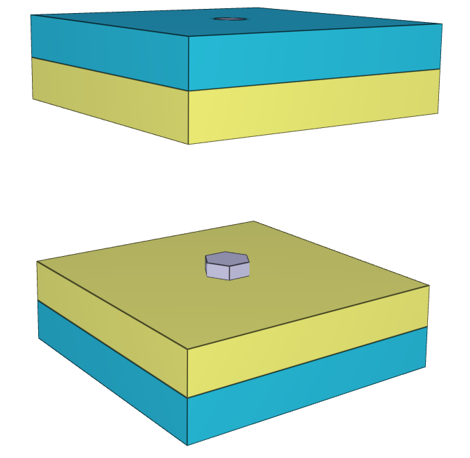
In Step 1 the bolts are prestressed to an axial stress (${\sigma_{pre}}$) of $100 \ MPa$. The bolts have a diameter ($D$) of $10.0 \ mm$, and the combined (2 bolt-hole pairs) total axial prestress force ($N$) should be $31.4 \ kN$.
In Step 2, the state files impetus_state1.k and impetus_state_bolt1.k are included from step 1. The bolts are automatically merged to the respective plates. There will be a slight redistribution of stresses.
Total force vs. time between the contact interfaces is presented in Figure 2 and 3
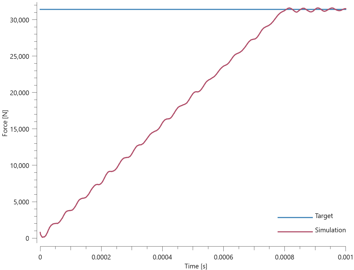
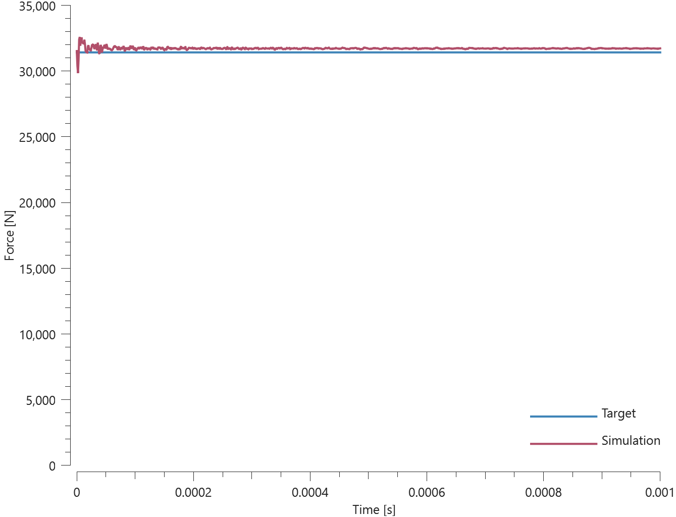
Contact forces and the pairing of bolts-plates is checked for version control.
Tests
This benchmark is associated with 2 tests.
*PRESTRESS_BOLT
Bolt assembly
pid${}_{bolt}$, pid${}_{nut}$, cid, $sf$, $t_{beg}$, $t_{end}$, no_match
This tests the *PRESTRESS_BOLT command. In this benchmark, the prestress functionality for a set of 10 bolts. All bolts are modelled by *COMPONENT_BOLT. The bolts connect two rings and a plate between them as seen in Figure 1.
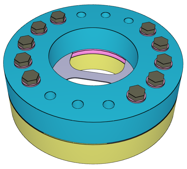
In Step 1, the bolts are prestressed to an axial stress ($\sigma_{pre}$) of $100 \ MPa$. The bolts have a diameter ($D$) of $15.9 \ mm$, and the total axial prestress force, $N$ should be $397.1 \ kN$.
In Step 2, the restart file from Step 1 is included, and the nuts are merged to the bolts.
Force vs. time between different contact interfaces are presented in Figure 2 and 3. The contact force between the bolts and the washers are checked for version control.
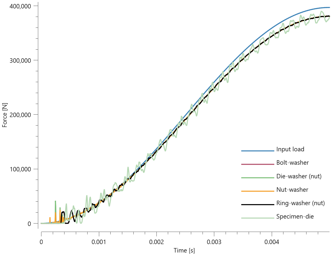
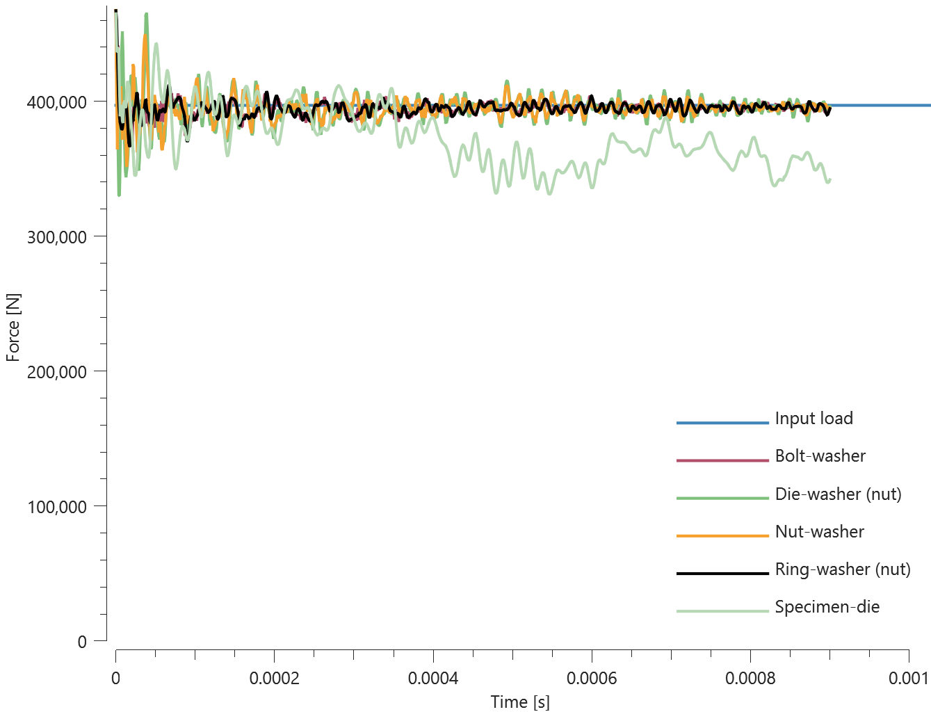
Tests
This benchmark is associated with 2 tests.
Double bolt
pid${}_{bolt}$, pid${}_{nut}$, cid, $sf$, $t_{beg}$, $t_{end}$, no_match
This tests the *PRESTRESS_BOLT command. In this benchmark, the prestress functionality is tested for two bolts. The bolts are modelled by *COMPONENT_BOLT and the test model is presented in Figure 1.

In Step 1 the bolts are prestressed to an axial stress ($\sigma_{pre}$) of $100 \ MPa$. The bolts have a diameter ($D$) of $28 \ mm$, and the total axial prestress force ($F$) for both bolts should be $123.2 \ kN$.
In Step 2, the restart file from Step 1 is included and the nuts are fixed to the bolts by activating the *MERGE command. There will be a slight redistribution of stresses when going from *PRESTRESS_BOLT to *MERGE. The contact force level will change and the error is proportional to the contact penalty stiffness. A smaller stiffness will produce smaller contact force errors.
Force vs. time between the plates are presented in Figure 2 and 3. The contact force between the two plates are checked for version control.
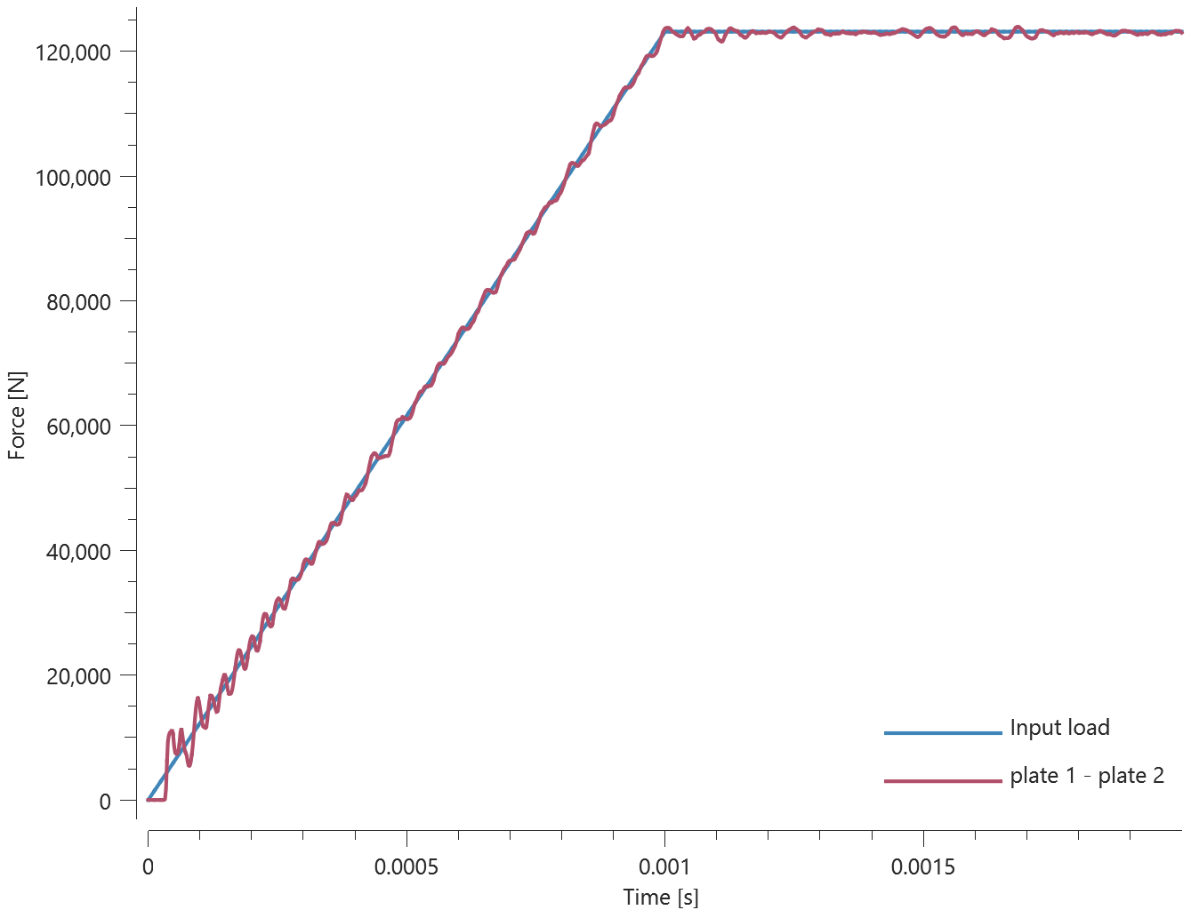
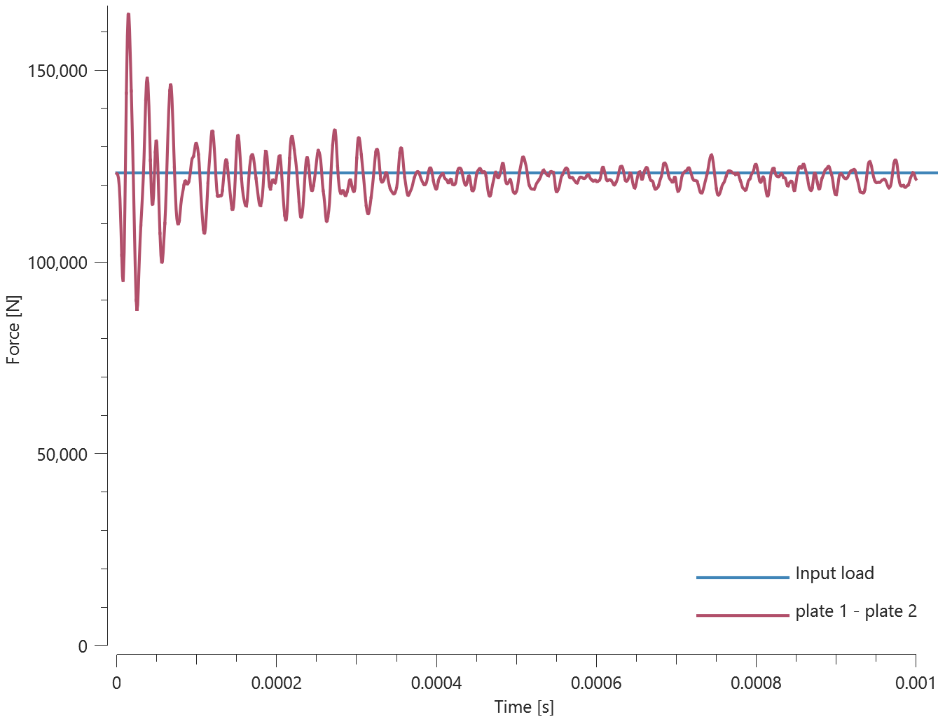
Tests
This benchmark is associated with 2 tests.
Single bolt
pid${}_{bolt}$, pid${}_{nut}$, cid, $sf$, $t_{beg}$, $t_{end}$, no_match
This tests the *PRESTRESS_BOLT command. In this benchmark, the prestress functionality is tested for a single bolt. The bolt is modelled by *COMPONENT_BOLT and the test model is displayed in Figure 1.
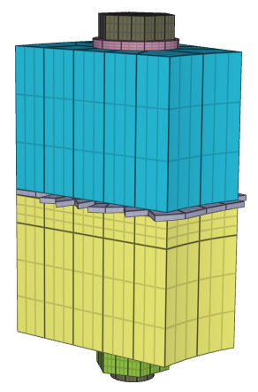
In Step 1 the bolt is prestressed to an axial stress (${\sigma_{pre}}$) of $200 \ MPa$. The bolt has a diameter ($D$) of $15.9 \ mm$, and the total axial prestress force ($N$) should be $39.7 \ kN$.
In Step 2, the restart file from Step 1 is included and the nut is fixed to the bolt by activating the *MERGE command. There will be a slight redistribution of stresses when going from *PRESTRESS_BOLT (Step 1) to *MERGE (Step 2). The contact force level will change and the error is proportional to the contact penalty stiffness. A smaller stiffness will produce smaller contact force errors.
Force vs. time between different contact interfaces are presented in Figure 2 and 3. The contact force between the nut and the washer is checked for version control.
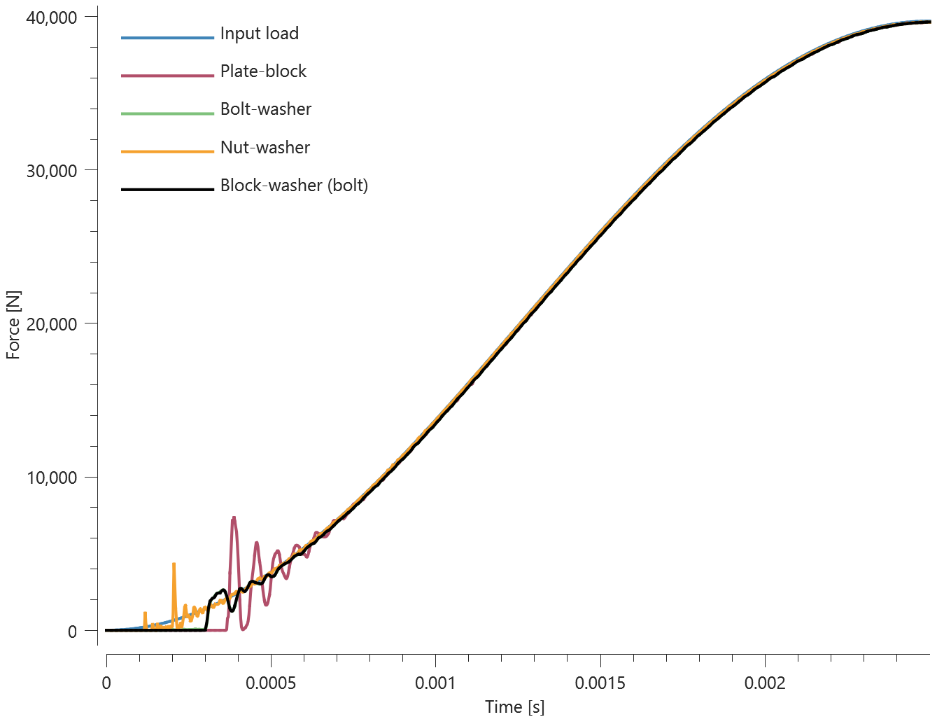
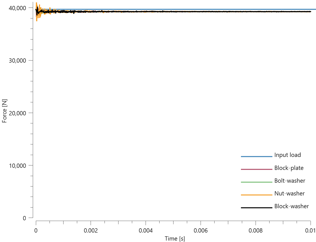
Tests
This benchmark is associated with 2 tests.
*PROP_DAMAGE_BRITTLE
Criterion test
"Optional title"
did, erode, noic
$\sigma_s$, $K_c$, $t_s$, $\alpha_s$, $\beta_s$
The failure criterion *PROP_DAMAGE_BRITTLE is verified in this test.
Tested parameters: $\sigma_s$, $t_s$, $\alpha_s$ and $\beta_s$.
Four CHEX elements are used in this test. Type of loading and type of threshold stress used in the failure criterion for each element is presented in Table 1.
| Element ID | Type of loading (Uniaxial) | Type of threshold stress |
|---|---|---|
| 1 | tension | First principal stress |
| 2 | compression | First principal stress |
| 3 | tension | First deviatoric principal stress |
| 4 | compression | First deviatoric principal stress |
The elements are loaded to a target stress, $\sigma_{vM}^t$ (effective value), and then kept at this stress level throughout the simulation.
For the investigated loading conditions, the first principal stress and first deviatoric principal stress are related to the target stress as presented in Table 2.
| Stress state (uniaxial) | First principal stress, $\sigma_1$ | First deviatoric principal stress, $\sigma_1^{dev}$ |
|---|---|---|
| tension | $\sigma_1 = \sigma_{vM}^t$ | $\sigma_1^{dev} = \frac{2}{3} \sigma_{vM}^ t$ |
| compression | $\sigma_1 = 0.0$ | $\sigma_1^{dev} = \frac{1}{3} \sigma_{vM}^ t$ |
Both the first principal stress and the first deviatoric principal stress exceeds the threshold stress, $\sigma_s$, in the case of tension, but not in compression. This means that damage starts to develop in the elements in tension, while the elements in compression remains intact. The times to develop fracture for the elements in tension are calculated as:
$$ t_1 = \frac{t_s}{(\sigma_1/\sigma_s)^{\alpha_s}} $$
$$ t_2 = \frac{t_s}{(\sigma_1^{dev}/\sigma_s)^{\alpha_s}} $$
$t_2$ is used as termination time. Damage vs. time in each element is presented in Figure 1 - 4 together with target curves from a verification script.
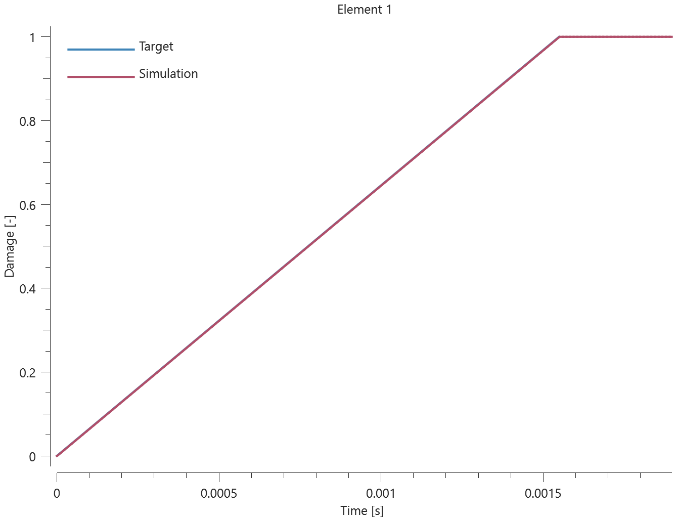

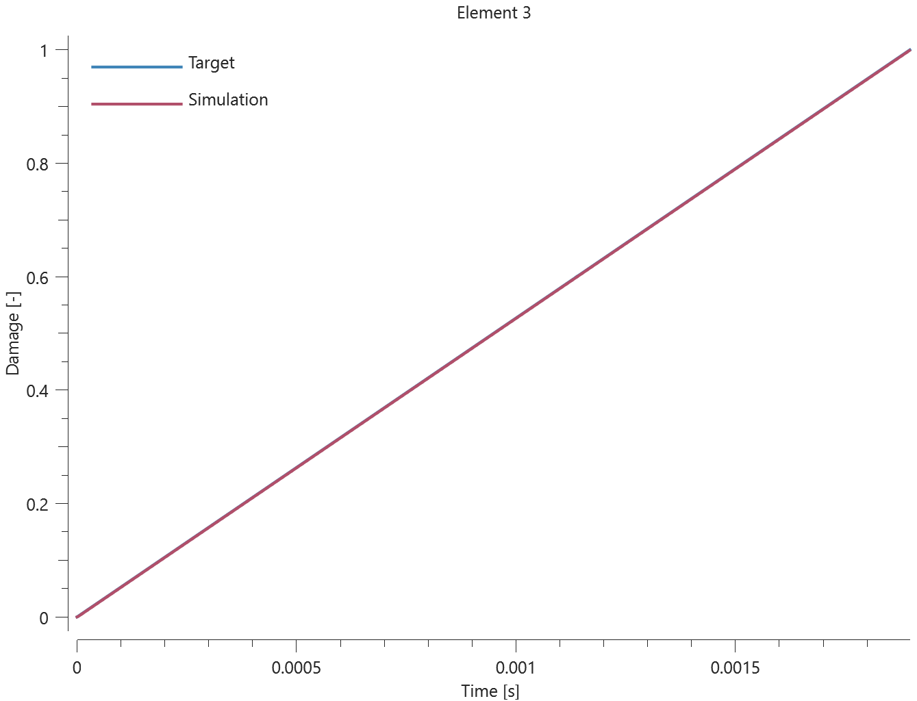

Maximum and average damage are checked in the elements.
Tests
This benchmark is associated with 1 tests.
*PROP_DAMAGE_CL
Brittle criterion test
"Optional title"
did, erode, noic
$W_c$, $G_I$, $\sigma_s$, $t_s$, $\alpha_s$, $\beta_s$
This test is identical to the test used to verify *PROP_DAMAGE_BRITTLE with the exception that *PROP_DAMAGE_CL is used instead.
Tested parameters: $\sigma_s$, $t_s$, $\alpha_s$ and $\beta_s$.
Damage vs. time in each element is presented in Figure 1 - 4 together with target curves from a verification script.


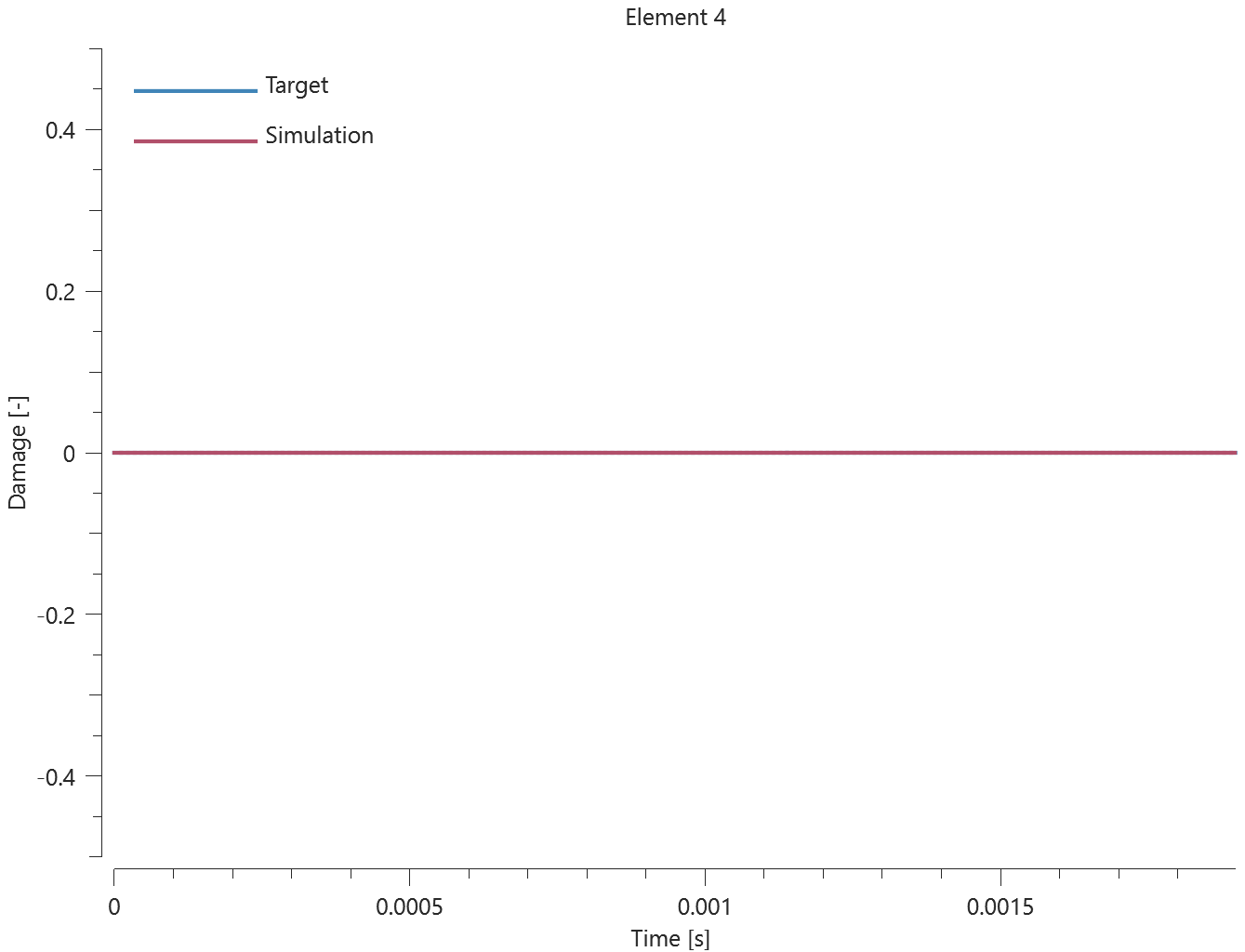
Maximum and average damage are checked in the elements.
Tests
This benchmark is associated with 1 tests.
Ductile criterion test
"Optional title"
did, erode, noic
$W_c$, $G_I$, $\sigma_s$, $t_s$, $\alpha_s$, $\beta_s$
The ductile failure criterion in *PROP_DAMAGE_CL is verified in this test.
Tested parameter: $W_c$.
A CHEX element is loaded in uniaxial tension. Damage vs. effective plastic strain from the simulation is displayed in Figure 1 together with a target curve from a verification script.

Maximum and average damage are checked.
Tests
This benchmark is associated with 1 tests.
Pressure smoothing
"Optional title"
did, erode, noic
$W_c$, $G_I$, $\sigma_s$, $t_s$, $\alpha_s$, $\beta_s$
This tests the pressure smoothing parameter. A hollow cylinder is given an initial velocity and dropped onto a surface. The damage in the bottom of the cylinder is then evaluated. The result is compared to the result from the same simulation, but with the pressure smoothing option turned off.
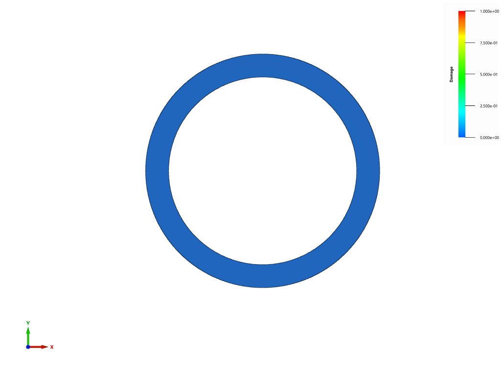
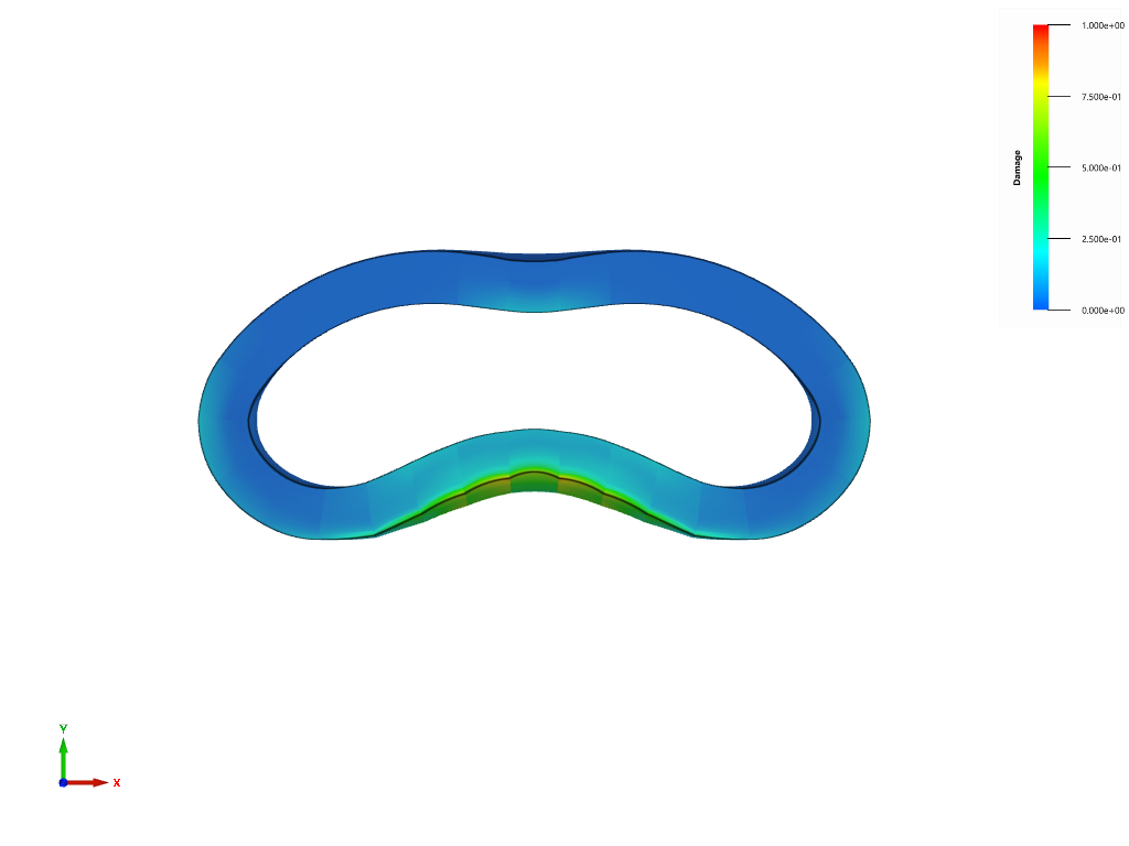
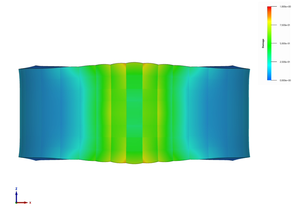

Comparing the result in Figure 3 and Figure 4, it can be seen that the pressure smoothing gives a more even distribution of the damage. The damage is also overallt lower with pressure smoothing than without.
The maximum obtained damage is checkat at two senosors at the bottom of the model.
*PROP_DAMAGE_CL_0_45_90
Criterion test (global coordinate system)
"Optional title"
did, erode, noic
$W_{0}$, $W_{45}$, $W_{90}$
The anisotropic failure criterion *PROP_DAMAGE_CL_0_45_90 is verified in this test.
Tested parameters: $W_0$, $W_{45}$ and $W_{90}$.
Three CHEX elements, defined in the global coordinate system, are loaded in uniaxial tension. Material orientations are defiend by *INITIAL_MATERIAL_DIRECTION_VECTOR. Initial material directions expressed in global coordinate axes for each element are presented in Table 1.
| Element ID | Local x-axis, [X,Y,Z] | Local y-axis, [X,Y,Z] |
|---|---|---|
| 1 | [1, 0, 0] | [0, 1, 0] |
| 2 | [$1 / \sqrt{2}, \ 1 / \sqrt{2}, \ 0$] | [$-1/\sqrt{2}, \ 1/\sqrt{2}, \ 0$] |
| 3 | [0, 1, 0] | [-1, 0, 0] |
Damage vs. effective plastic strain in the elements are compared to target curves from a verification script in Figure 1.
/prop_damage_cl_0_45_90_fracture_criterion_global_cs.png)
Maximum and average damage are checked in the elements.
Tests
This benchmark is associated with 1 tests.
Criterion test (local coordinate system)
"Optional title"
did, erode, noic
$W_{0}$, $W_{45}$, $W_{90}$
This test is similar to "*PROP_DAMAGE_CL_0_45_90 - Criterion test (global coordinate system)". The difference is that in this test, the elements and loads are defined in a local coordinate system with the z-axis rotated 45° around the global Z-axis.
Material directions are still defined in the global system. Loading directions and material directions relate to each other in the same way as in the aforementioned test, meaning that the same damage vs. effective plastic strain curves from the elements are expected.
Damage vs. effective plastic strain in the elements are compared to target curves from a verification script in Figure 1.
/prop_damage_cl_0_45_90_fracture_criterion_local_cs.png)
Maximum and average damage are checked in the elements.
Tests
This benchmark is associated with 1 tests.
*PROP_DAMAGE_CL_ANISOTROPIC
Criterion test (global coordinate system)
"Optional title"
did, erode, noic
$W_{0}$, $W_{90}$, $W_{t}$
The anisotropic failure criterion *PROP_DAMAGE_CL_ANISOTROPIC is verified in this test.
Tested parameters: $W_0$, $W_{90}$ and $W_{t}$.
Three CHEX elements, defined in the global coordinate system, are loaded in uniaxial tension. Material orientations are defiend by *INITIAL_MATERIAL_DIRECTION_VECTOR. Initial material directions expressed in global coordinate axes for each element are presented in Table 1.
| Element ID | Local x-axis, [X,Y,Z] | Local y-axis, [X,Y,Z] |
|---|---|---|
| 1 | [1, 0, 0] | [0, 1, 0] |
| 2 | [0, 1, 0] | [-1, 0, 0] |
| 3 | [0, 0, 1] | [0, 1, 0] |
Damage vs. effective plastic strain in the elements are compared to target curves from a verification script in Figure 1.
/prop_damage_cl_anisotropic_fracture_criterion_global_cs.png)
Maximum and average damage are checked in the elements.
Tests
This benchmark is associated with 1 tests.
Criterion test (local coordinate system)
"Optional title"
did, erode, noic
$W_{0}$, $W_{90}$, $W_{t}$
This test is similar to "*PROP_DAMAGE_CL_ANISOTROPIC - Criterion test (global coordinate system)". The difference is that in this test, the elements and loads are defined in a local coordinate system. The local coordinate system is first rotated 45° around the global Z-axis and then -45° around the local y-axis.
Material directions are still defined in the global system. Loading directions and material directions relate to each other in the same way as in the aforementioned test, meaning that the same damage vs. effective plastic strain curves from the elements are expected.
Damage vs. effective plastic strain in the elements are compared to target curves from a verification script in Figure 1.
/prop_damage_cl_anisotropic_fracture_criterion_local_cs.png)
Maximum and average damage are checked in the elements.
Tests
This benchmark is associated with 1 tests.
*PROP_DAMAGE_CL_REGULARIZE
Regularize feature
"Optional title"
did, erode, noic
$W_c$, $R_0$, $D_0$, $c$
The regularization feature in *PROP_DAMAGE_CL_REGULARIZE is verified in this test.
Tested parameters: $R_0$, $D_0$ and $c$.
Regularization is a feature that reduces the mesh dependency in the damage model. The feature is useful in models where material fails in tension and where elements have significantly larger in-plane dimensions compared to the thickness.
The model consists of four rectangular specimens with thickness t, width 8t and length 16t. Four different meshes are used in the specimens, as displayed in Figure 1. The number of CHEX elements used in the specimens are presented in Table 1.
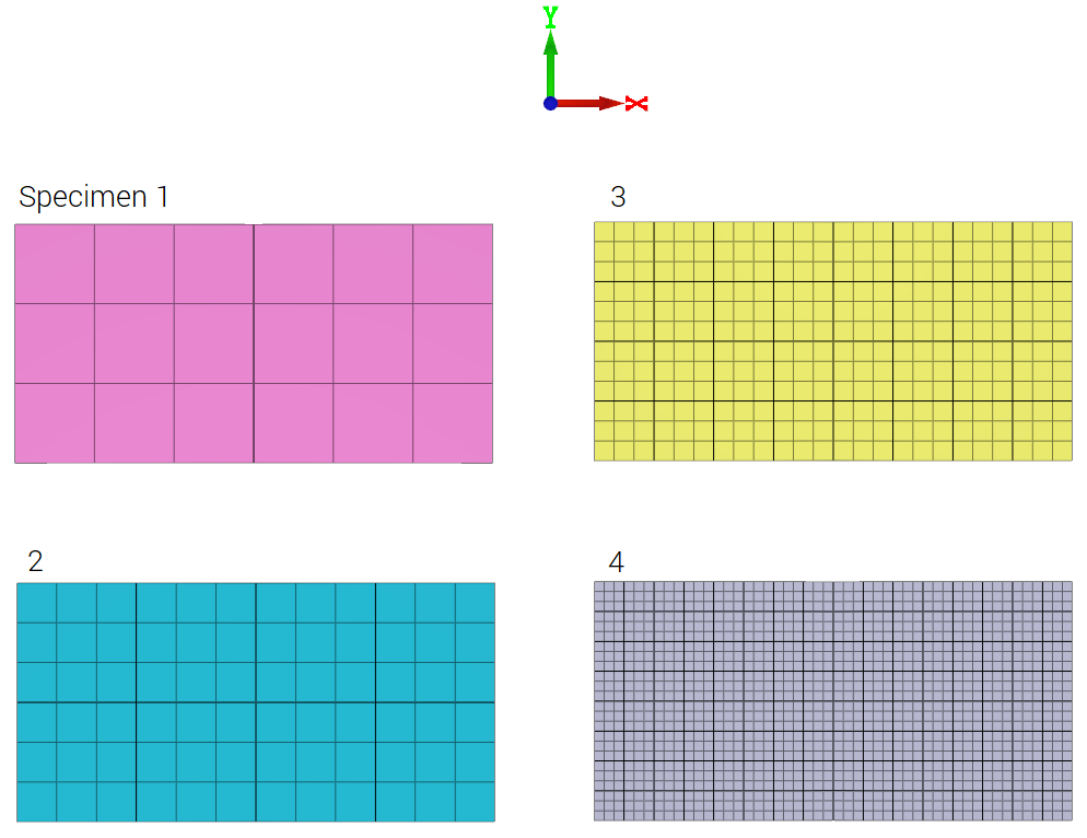
| Specimen ID | X-dir. | Y-dir. | Z-dir. |
|---|---|---|---|
| 1 | 2 | 1 | 1 |
| 2 | 4 | 2 | 1 |
| 3 | 8 | 4 | 1 |
| 4 | 16 | 8 | 1 |
Material and damage properties are the same in the four specimens and the same prescribed motion is imposed, which causes a state of uniaxial tension in the specimens. The model is run with *PROP_DAMAGE_CL and with *PROP_DAMAGE_CL_REGULARIZE to illustrate the regularization feature. Regularization parameters are optimized through the metal calibration project.
Damage vs. time for all specimens are presented in Figure 2 and 3. Figure 2 shows the results with *PROP_DAMAGE_CL, which is without regularization, and Figure 3 the results with *PROP_DAMAGE_CL_REGULARIZE, which is with regularization.
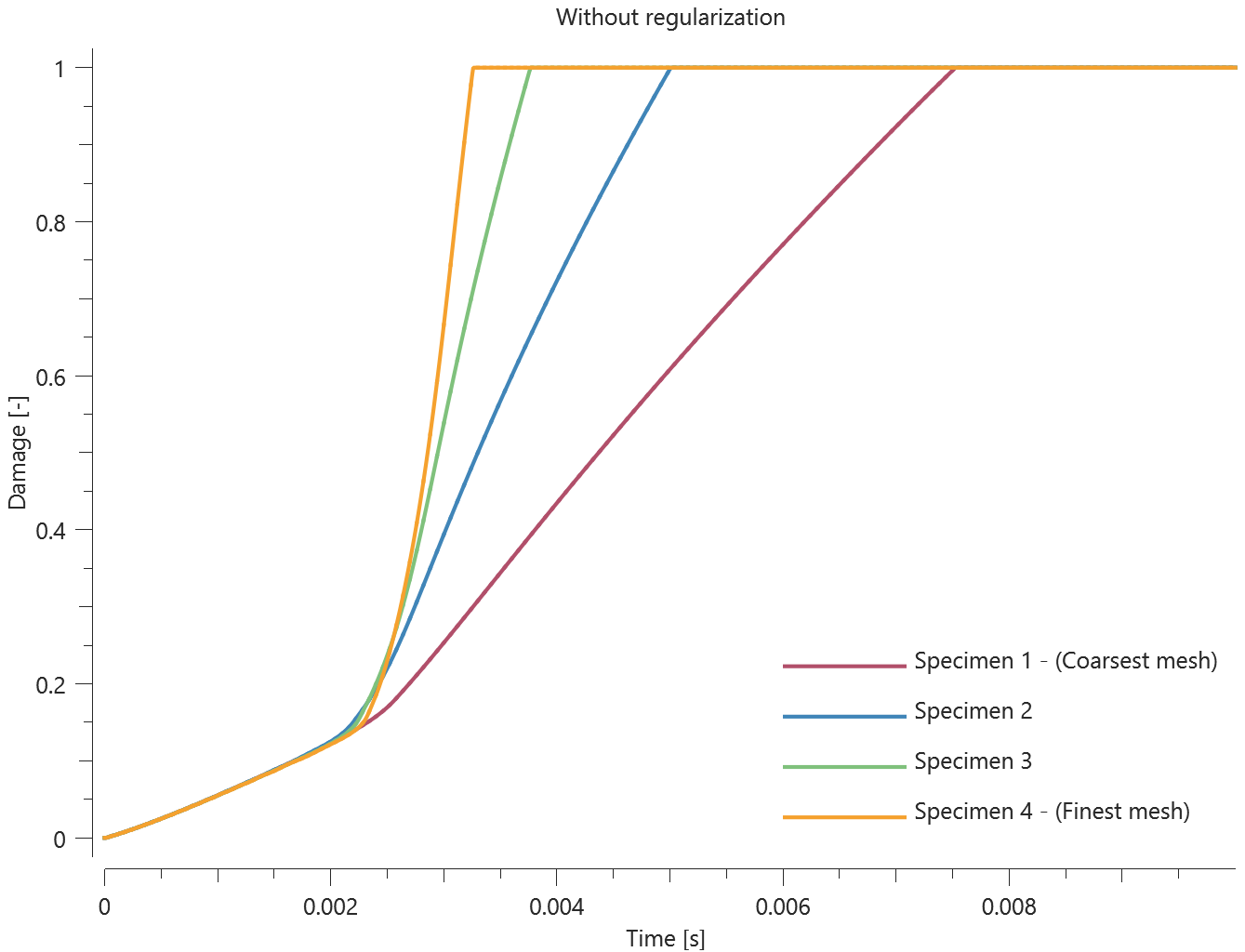
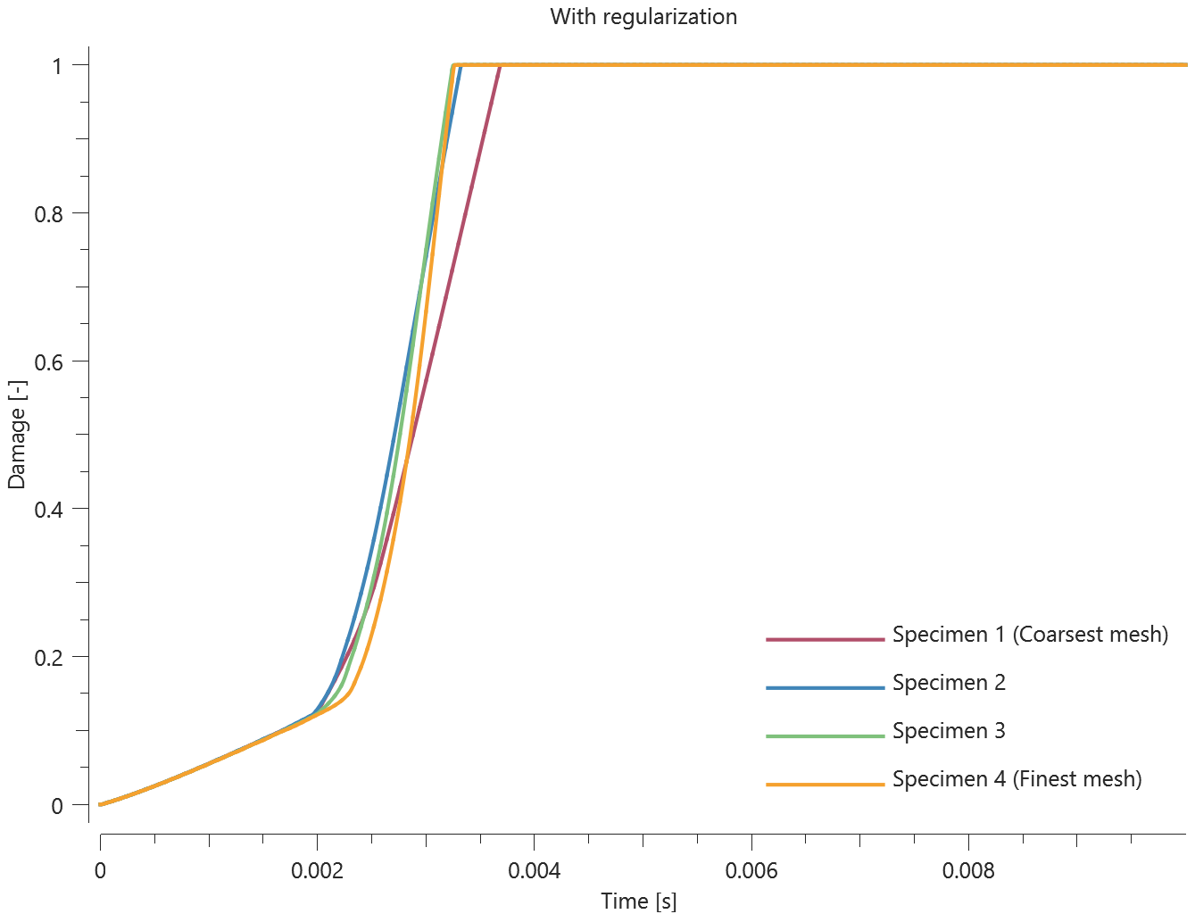
Figure 4 shows damage vs. time for the coarsest and the finest mesh for both damage models. Note that the regularize feature does not have any effect in the finest mesh, and therefore the curves with and without regularization are identical.
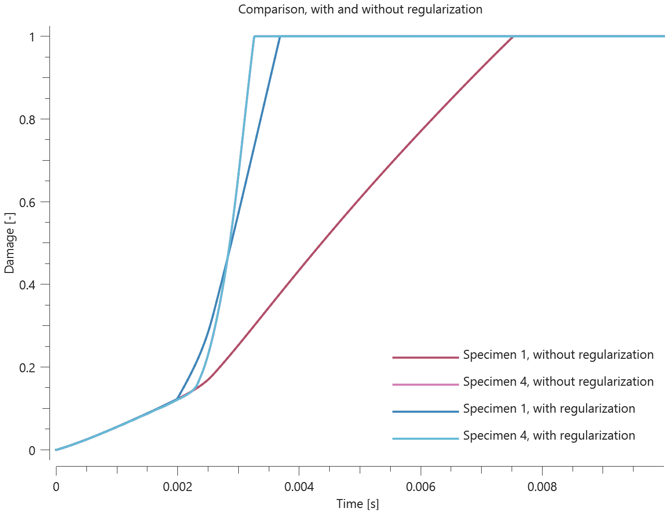
Maximum and average damage in the specimens are checked for version control.
Tests
This benchmark is associated with 2 tests.
*PROP_DAMAGE_GOLDTHORPE
Criterion test
"Optional title"
did, erode, noic
$S$, $A$
The failure criterion *PROP_DAMAGE_GOLDTHORPE is verified in this test.
Tested parameters: S and A.
The model consist of two cubes, each modeled with a single LHEX element. Prescribed strain rates are imposed on the cubes, causing a state of uniaxial tensile stress in one of the cubes, and a state of uniaxial compressive stress in the other.
Damage vs. effective plastic strain from the two elements are presented in Figure 1 and Figure 2 together with target curves obtained from another numerical approach.
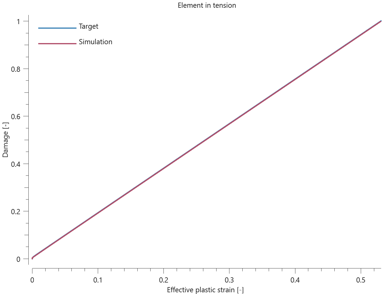
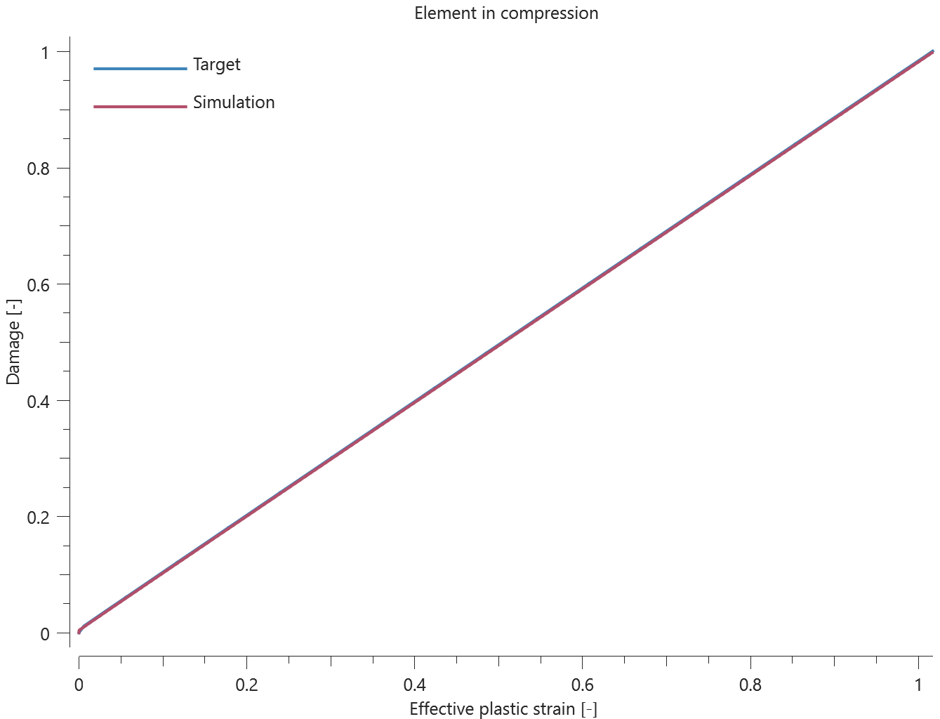
Maximum and average damage are checked in both elements.
Tests
This benchmark is associated with 1 tests.
*PROP_DAMAGE_HC
Brittle criterion test
"Optional title"
did, erode, noic
$a$, $b$, $c$, $n$, $T_a$, $T_b$, $\sigma_s$, $t_s$
$\alpha_s$, $c_r$, $\dot\varepsilon_r$, $G_I$
The brittle failure criterion in *PROP_DAMAGE_HC is verified in this test.
Tested parameters: $\sigma_s$, $t_s$ and $\alpha_s$.
A CHEX element is subjected to a cyclic uniaxial load. The amplitude of the load is increasing with time. Damage vs. time in the element is presented in Figure 1 together with a target curve from a verification script.
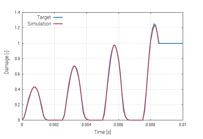
Maximum and average damage are checked.
Tests
This benchmark is associated with 1 tests.
Ductile criterion test (triaxiality, Lode parameter and thermal dependency)
"Optional title"
did, erode, noic
$a$, $b$, $c$, $n$, $T_a$, $T_b$, $\sigma_s$, $t_s$
$\alpha_s$, $c_r$, $\dot\varepsilon_r$, $G_I$
The ductile failure criterion in *PROP_DAMAGE_HC is verified in this test.
Tested parameters: $a$, $b$, $c$, $n$, $T_a$ and $T_b$.
Five CHEX elements are subjected to different states of stress. Lode parameters and triaxialities associated with the stress states are presented in Table 1.
| Element ID | Stress state | Lode parameter | Triaxiality |
|---|---|---|---|
| 1 | Biaxial compression | 1 | -2/3 |
| 2 | Biaxial tension | -1 | 2/3 |
| 3 | Shearing | 0 | 0 |
| 4 | Uniaxial compression | -1 | -1/3 |
| 5 | Uniaxial tension | 1 | 1/3 |
The Lode parameter, $\theta$, is calculated as:
$$ \theta = 1 - \frac{2}{\pi} \cdot acos\left(3 \cdot \frac{\sqrt{3}}{2} \cdot \frac{J_3}{(J_2)^{3/2}}\right) $$
where $J_2$ and $J_3$ is the second and third invariant of the deviatoric stress tensor.
The triaxiality, $\eta$, is calculated as:
$$ \eta = \frac{I_1}{3 \cdot \sqrt{3J_2}} $$
where $I_1$ is the first invariant of the stress tensor.
Damage vs. effective plastic strain in the elements are presented in Figure 1 - 5 together with target curves from a verification script.
/prop_damage_hc_ductile_biaxial_compression.png)
/prop_damage_hc_ductile_biaxial_tension.png)
/prop_damage_hc_ductile_shearing.png)
/prop_damage_hc_ductile_uniaxial_compression.png)
/prop_damage_hc_ductile_uniaxial_tension.png)
Maximum and average damage are checked in the elements.
Tests
This benchmark is associated with 1 tests.
*PROP_DAMAGE_IMP
Criterion test
"Optional title"
did, erode, noic
$W_c$, $n$
The failure criterion *PROP_DAMAGE_IMP is verifed in this test.
Tested parameters: $W_c$ and $n$.
A CHEX element is loaded in uniaxial tension. Damage vs. effective plastic strain in the element is dislayed in Figure 1 together with a target curve obtained from a verification script.
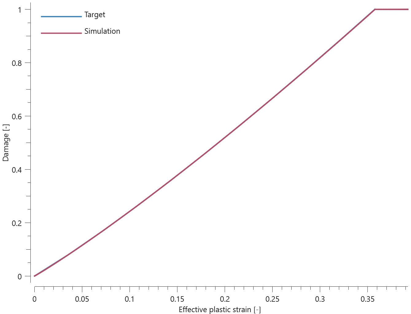
Maximum and average damage are checked.
Tests
This benchmark is associated with 1 tests.
*PROP_DAMAGE_IMP_ISO
Criterion test
"Optional title"
did, erode, noic
$A_{imp}$, $B_{imp}$, $W_{imp}$
The failure criterion *PROP_DAMAGE_IMP_ISO is verified in this test.
Tested parameters: $A_{imp}$, $B_{imp}$ and $W_{imp}$.
A CHEX element is loaded in uniaxial tension. Both $A_{imp}$ and $B_{imp}$ are defined, meaning that both terms of the failure criterion are activated. Damage vs. effective plastic strain in the element is displayed in Figure 1 together with a target curve from a verification script.
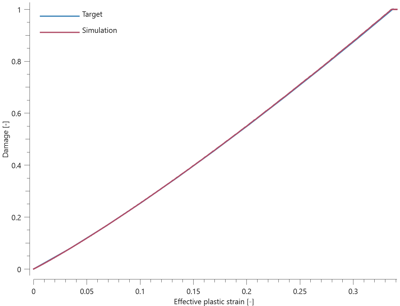
Maximum and average damage are checked.
Tests
This benchmark is associated with 1 tests.
*PROP_DAMAGE_JC
Criterion test (minimum failure strain)
"Optional title"
did, erode, noic
$d_1$, $d_2$, $d_3$, $d_4$, $d_5$, $\dot\varepsilon_0$, $T_0$, $T_m$
$\varepsilon_{min}$
The minimum failure strain in the failure criterion *PROP_DAMAGE_JC is verified in this test.
Tested parameter: $\varepsilon_{min}$.
This test is similar to "*PROP_DAMAGE_JC - Criterion test (triaxiality, strain rate and thermal dependency)". The only difference is that a minimum failure strain is added in this test.
Damage vs. effective plastic strain from the elements is presented in Figure 1 - 3 together with target curves from a verification script.
/prop_damage_jc_minimum_failure_strain_uniaxial_tension.png)
/prop_damage_jc_minimum_failure_strain_uniaxial_compression.png)
/prop_damage_jc_minimum_failure_strain_shearing.png)
Maximum and average damage are checked in the elements.
Tests
This benchmark is associated with 1 tests.
Criterion test (triaxiality, strain rate and thermal dependency)
"Optional title"
did, erode, noic
$d_1$, $d_2$, $d_3$, $d_4$, $d_5$, $\dot\varepsilon_0$, $T_0$, $T_m$
$\varepsilon_{min}$
The triaxiality, strain rate dependency and thermal dependency in the failure criterion *PROP_DAMAGE_JC are verified in this test.
Tested parameters: $d_1$, $d_2$, $d_3$, $d_4$, $d_5$, $\dot\varepsilon_0$, $T_0$ and $T_m$.
The test consist of three CHEX elements, loaded in accordance to Table 1.
| Element ID | Type of loading | Triaxiality |
|---|---|---|
| 1 | Uniaxial tension | -1/3 |
| 2 | Uniaxial compression | 1/3 |
| 3 | Shearing | 0 |
Loading is done by a prescribed motion, causing a strain rate of $100 \ 1/s$. An initial temperature of $600 \ K$ is used in the elements and all tested parameters assumes non-zero values. This configuration ensures that all the tested parameters contribute to the failure strain.
Damage vs. effective plastic strain in the elements are presented in Figure 1 - 3 together with target curves from a verification script.
/prop_damage_jc_triaxiality_rate_thermal_dependency_uniaxial_tension.png)
/prop_damage_jc_triaxiality_rate_thermal_dependency_uniaxial_compression.png)
/prop_damage_jc_triaxiality_rate_thermal_dependency_shearing.png)
Maximum and average damage are checked in the elements.
Tests
This benchmark is associated with 1 tests.
*PROP_DAMAGE_JC_MODIFIED
Triaxiality and strain rate dependency
"Optional title"
did, erode, noic
$d_1$, $\varepsilon_c$, $\varepsilon_t$, $\alpha$
Tested parameters: $d_1$, $\varepsilon_{c}$, $\varepsilon_t$ and $\alpha$.
The model consists of four LHEX elements. A prescribed strain rate is imposed in the X-direction while the elements are unconstrained in the Y- and Z-direction, leading to a uniaxial stress state. Two of the elements are being compressed and the two are being stretched. Strain rate effects are included for one of the elements subjected to each type of loading.
| Element ID | Stress state | Strain rate effects |
|---|---|---|
| 1 | Uniaxial compression | Excluded |
| 2 | Uniaxial tension | Excluded |
| 3 | Uniaxial compression | Included |
| 4 | Uniaxial tension | Included |
Plots of effective stress vs. effective plastic strain and damage vs. effective plastic strain are presented in Figure 1 – 8 together with target curves obtained from a verification script. Note that element 2 and 4 generate the same response, since strain rate effects are only active for a positive pressure.
The model is run with the following input:
| $d_1$ = 0.1 | [-] | |
| $\varepsilon_c$ = 0.5 | [-] | |
| $\varepsilon_t$ = 0.05 | [-] | |
| $\alpha$ = 1e-3 | [s] | (Element 3 and 4) |
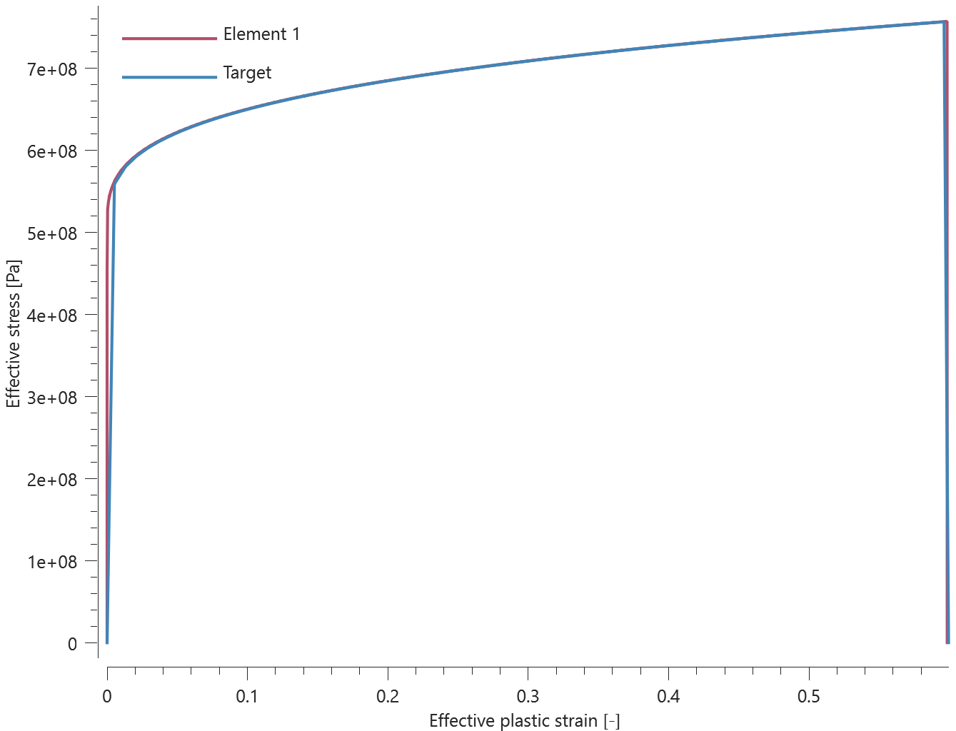
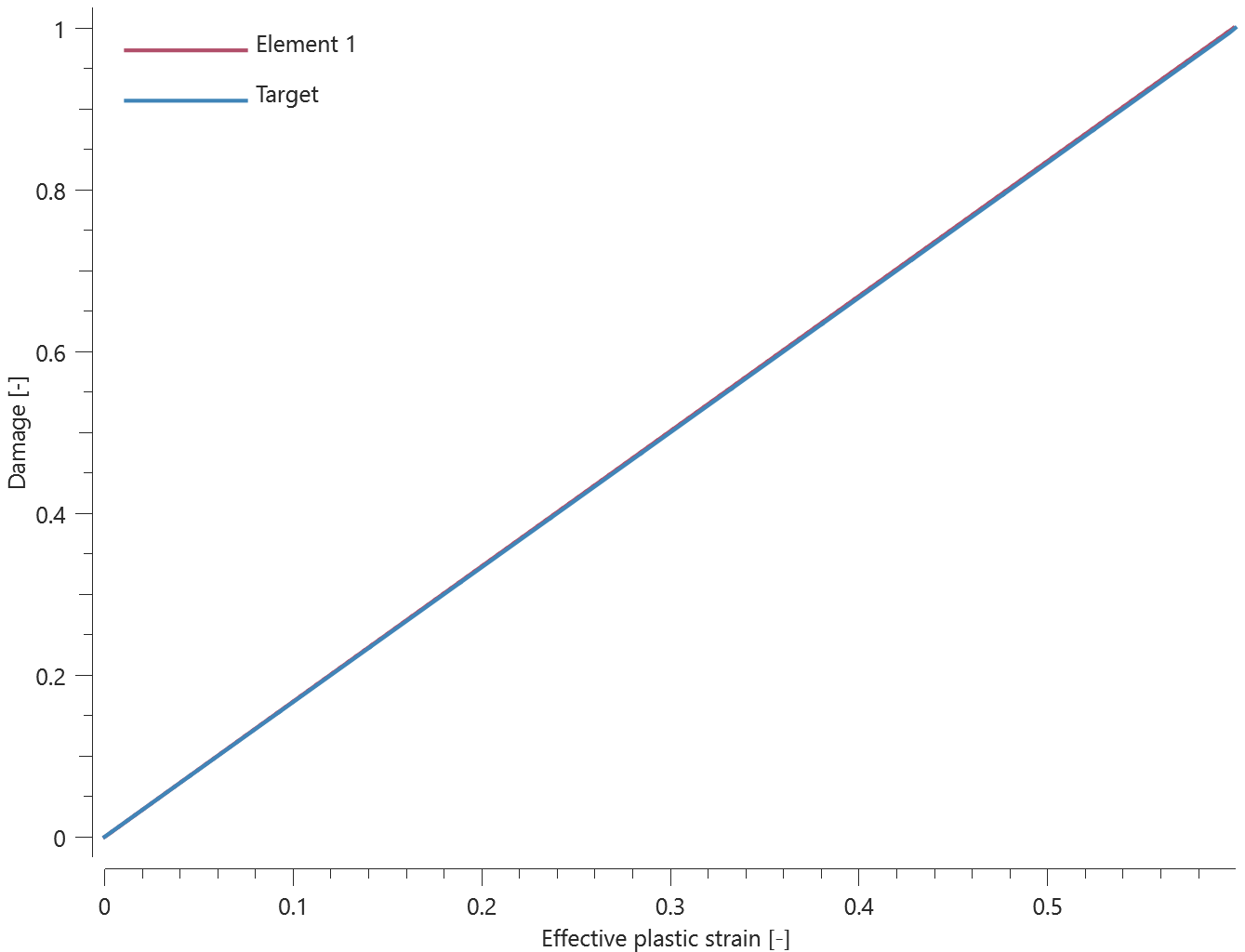

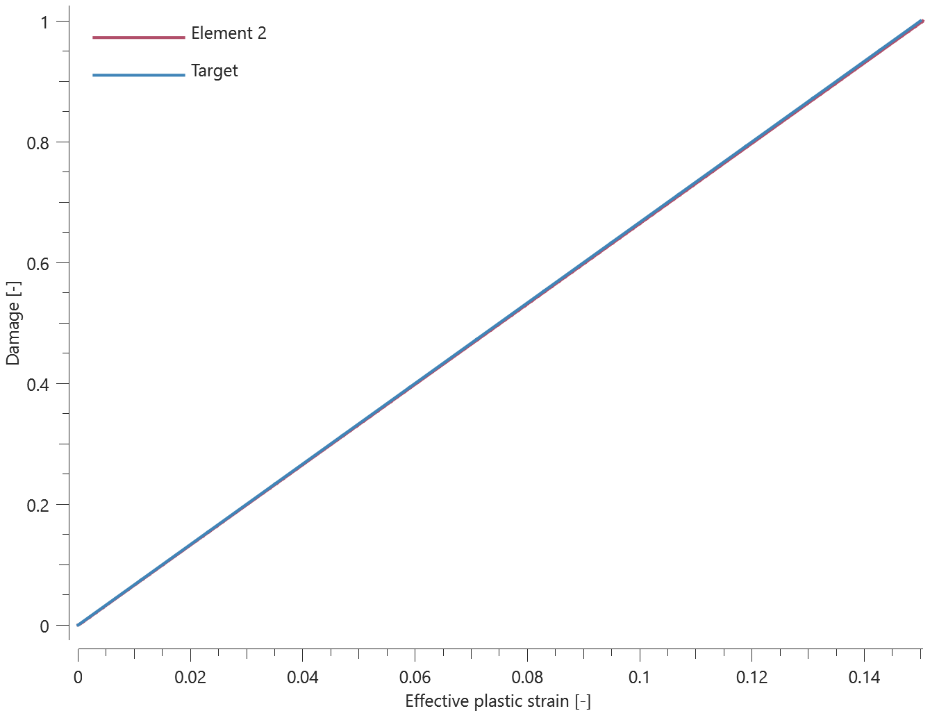
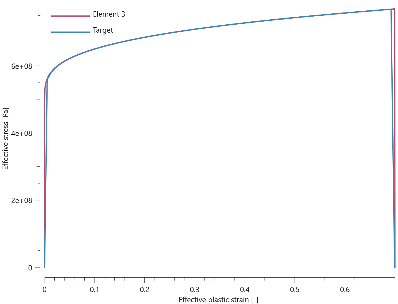
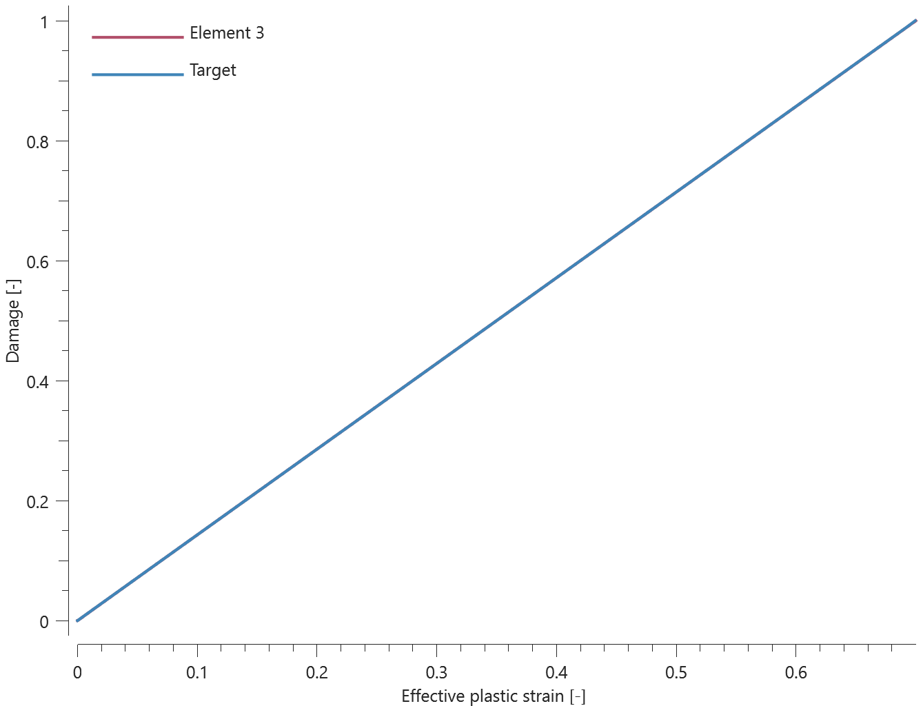
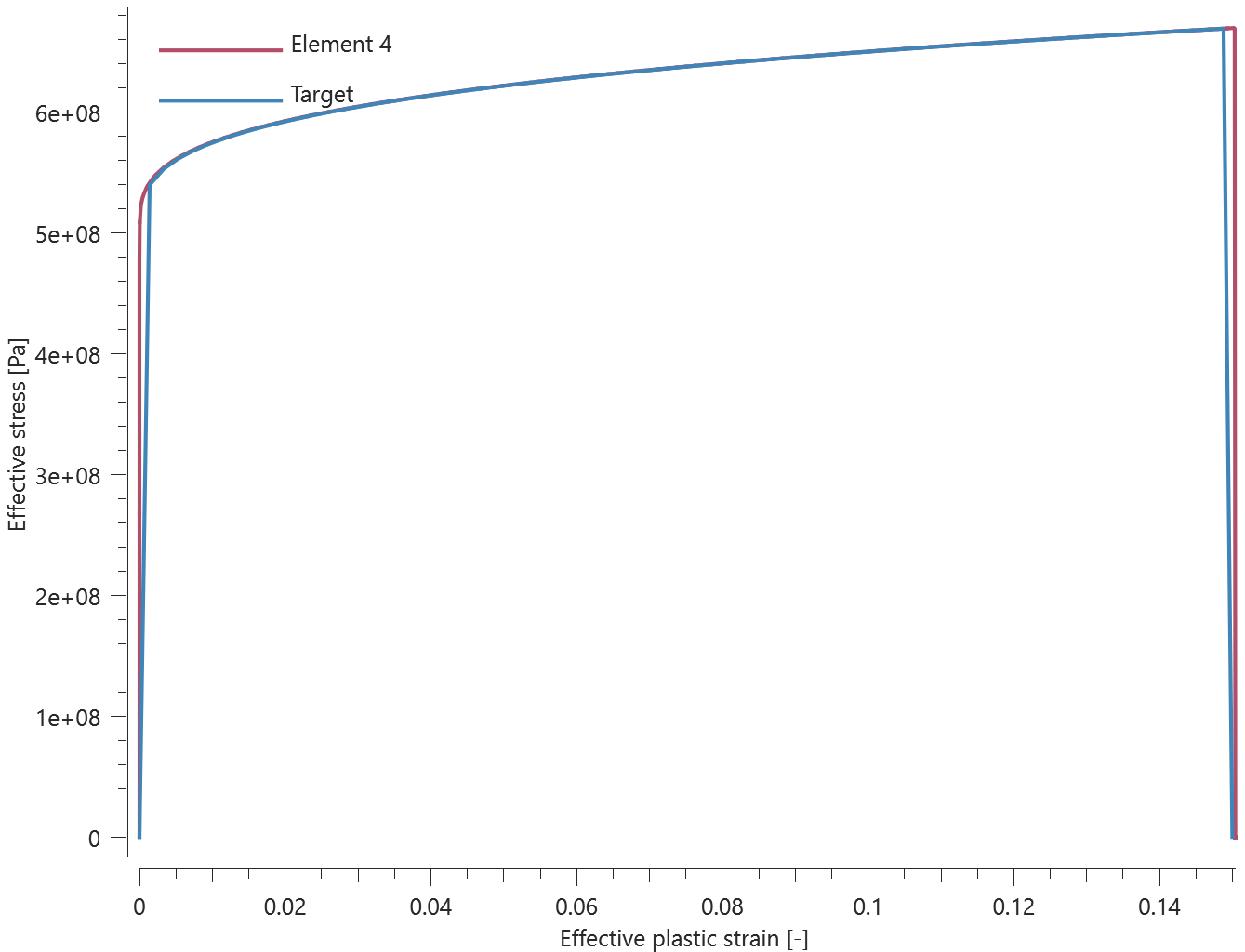
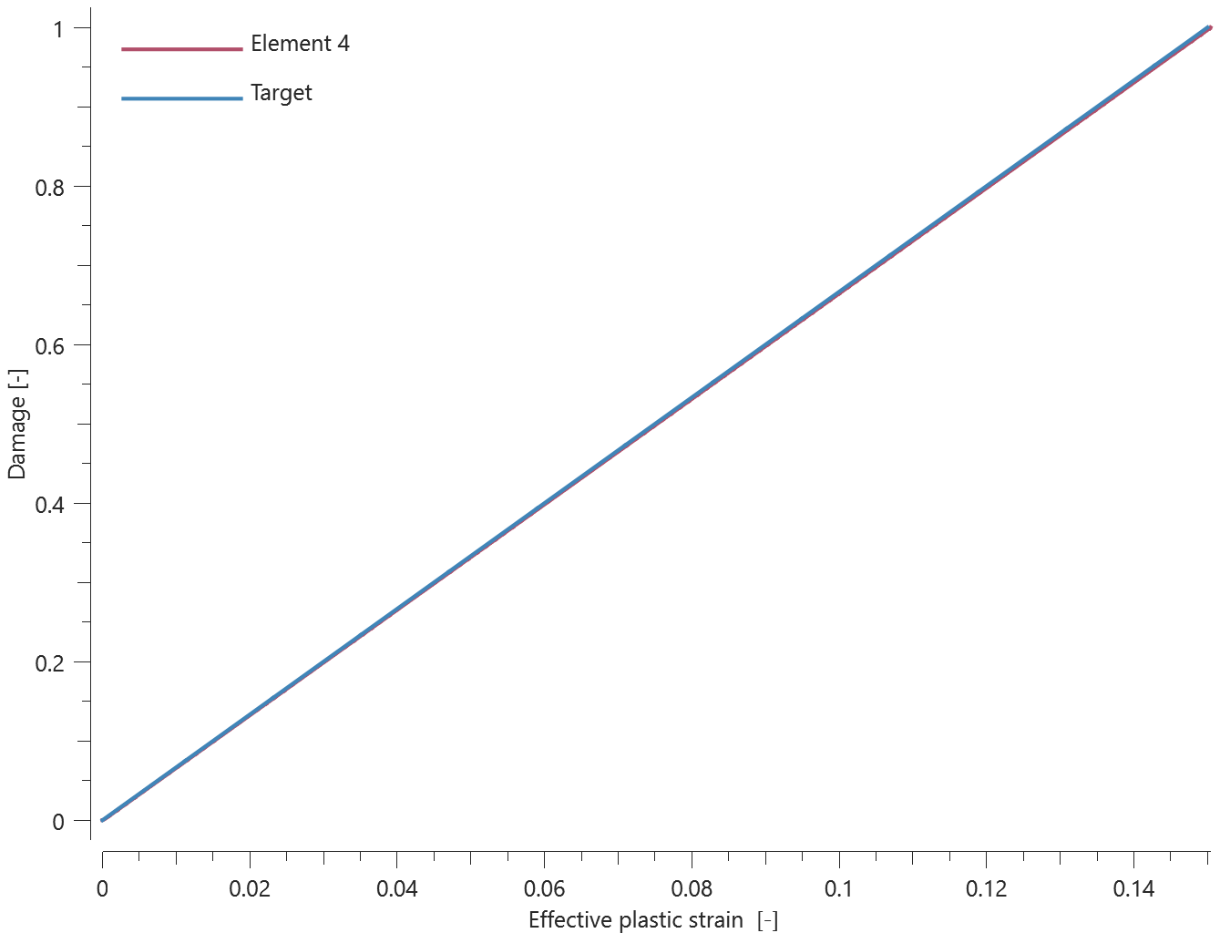
Last value of damage, effective plastic strain and effective stress as well as maximum value of effective stress is checked for the elements.
Tests
This benchmark is associated with 4 tests.
*PROP_DAMAGE_MTSB
Minimum failure strain
"Optional title"
did, erode, noic
$a$, $b$, $\alpha$, $\varepsilon_{min}$
Tested parameters: $\varepsilon_{min}$.
A LHEX element loaded as Element 2 in the test “Pressure and strain rate dependency” is used. A minimum failure strain of 0.45 is applied.
Plots of effective stress vs. effective plastic strain and damage vs. effective plastic strain are presented in Figure 1 – 2 together with target curves obtained from a verification script.
The model is run with the following input:
| $a$ = 0.5 | [-] | |
| $b$ = 5e-10 | [1/Pa] | |
| $\alpha$ = 1e-3 | [s] | (Element 3 and 4) |
| $\varepsilon_{min}$ = 0.45 | [-] |
Tests
This benchmark is associated with 1 tests.
Pressure and strain rate dependency
"Optional title"
did, erode, noic
$a$, $b$, $\alpha$, $\varepsilon_{min}$
Tested parameters: 𝑎, 𝑏 and $\alpha$.
The model consists of four LHEX elements. A prescribed strain rate is imposed in the X-direction while the elements are unconstrained in the Y- and Z-direction, leading to a uniaxial stress state. Two of the elements are being compressed and the two are being stretched. Strain rate effects are included for one of the elements subjected to each type of loading.
| Element ID | Stress state | Strain rate effects |
|---|---|---|
| 1 | Uniaxial compression | Excluded |
| 2 | Uniaxial tension | Excluded |
| 3 | Uniaxial compression | Included |
| 4 | Uniaxial tension | Included |
Plots of effective stress vs. effective plastic strain and damage vs. effective plastic strain are presented in Figure 1 – 8 together with target curves obtained from a verification script. Note that element 2 and 4 generate the same response, since strain rate effects are only active for a positive pressure.
The model is run with the following input:
| $a$ = 0.5 | [-] | |
| $b$ = 5e-10 | [1/Pa] | |
| $\alpha$ = 1e-3 | [s] | (Element 3 and 4) |
| $\varepsilon_{min}$ = 0 | [-] |
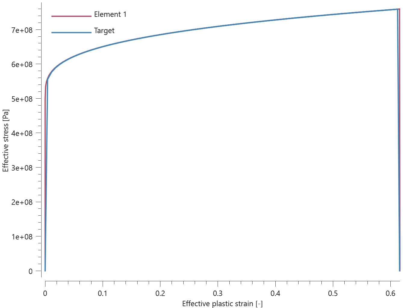
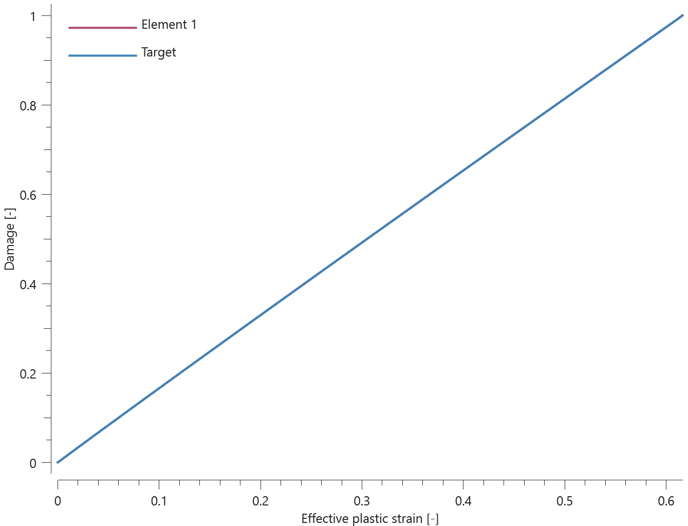
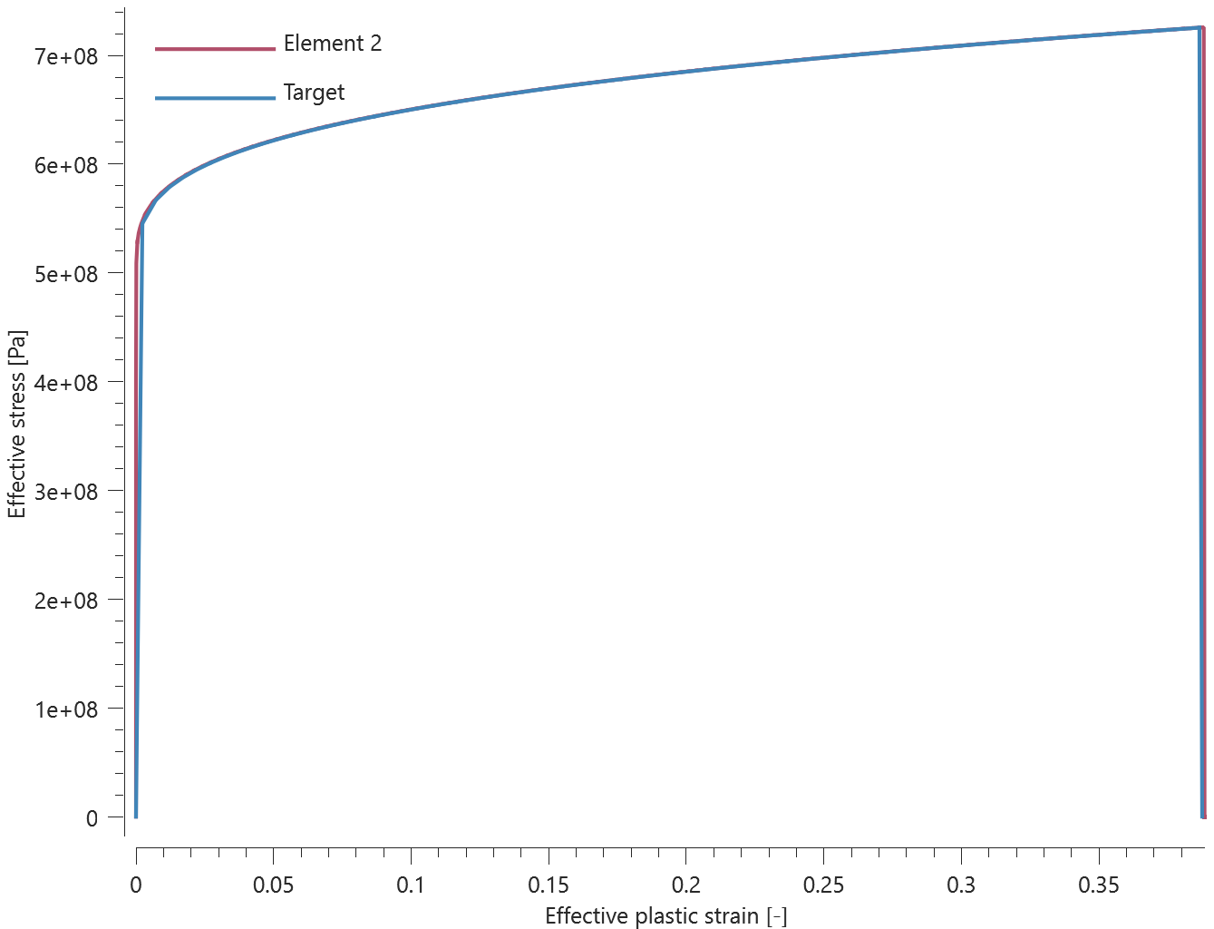


Last value of damage, effective plastic strain and effective stress as well as maximum value of effective stress is checked for the elements.
Tests
This benchmark is associated with 4 tests.
*PROP_DAMAGE_STRAIN
Criterion test
"Optional title"
did, erode, noic
$\varepsilon_{fail}^{geo}$, $\varepsilon_{fail}^{t}$, $\varepsilon_{fail}^{c}$, $\varepsilon_{fail}^{vol}$
The failure criterion *PROP_DAMAGE_STRAIN is verified in this test.
Tested parameters: $\varepsilon_{fail}^{geo}$, $\varepsilon_{fail}^{t}$, $\varepsilon_{fail}^{c}$ and $\varepsilon_{fail}^{vol}$.
Four CHEX elements are used in this test. Three of the elements are stretched while one is compressed. Deformation occurs in the Z-direction and the elements are fixed in the X- and Y-direction. The failure strain criterion used in each element, and the corresponding volumetric strain, is presented in Table 1.
| Element ID | Failure strain criterion | Volumetric strain at failure |
|---|---|---|
| 1 | $\varepsilon_{fail}^{geo}$ | $\sqrt{\frac{3}{2}} \cdot \varepsilon_{fail}^{geo}$ |
| 2 | $\varepsilon_{fail}^{t}$ | $\varepsilon_{fail}^{t}$ |
| 3 | $\varepsilon_{fail}^{c}$ | $\varepsilon_{fail}^{c}$ |
| 3 | $\varepsilon_{fail}^{vol}$ | $\varepsilon_{fail}^{vol}$ |
Damage vs. volumetric strain in the elements are presented in Figure 1 and 2 together with target curves from a verification script.
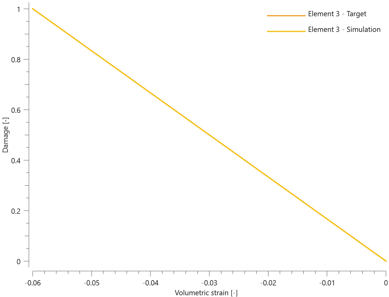
Maximum and average damage are checked in the elements.
Tests
This benchmark is associated with 1 tests.
*PROP_DAMAGE_XW
Criterion test
"Optional title"
did, erode, noic
$c_1$, $c_2$, $c_3$, $c_4$, $n$
The failure criterion *PROP_DAMAGE_XW is verified in this test.
Tested parameters: $c_1$, $c_2$, $c_3$, $c_4$ and $n$.
Four LHEX elements are subjected to the stress states as presented below.
| Element ID | Stress state | Stress triaxiality | Lode paramter | |||
|---|---|---|---|---|---|---|
| 1 | Uniaxial tension | 1/3 | 1 | |||
| 2 | Uniaxial compression | -1/3 | -1 | |||
| 3 | Biaxial tension | 2/3 | -1 | |||
| 4 | Biaxial compression | -2/3 | 1 |
The prescribed motions imposed on the elements are continuously increased until failure occurs. Damage vs effective plastic strain extracted from the elements are presented together with target curves in Figure 1.
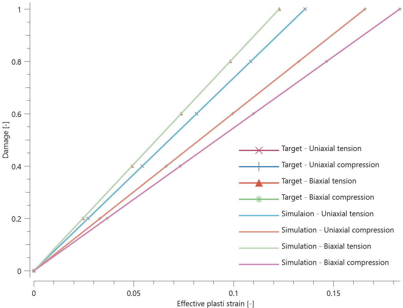
The last values of damage and effective plastic strain are checked.
Tests
This benchmark is associated with 1 tests.
*PROP_SPOT_WELD
Normal stress
"Optional title"
coid
$R$, $h$, $m$, $k$, $F_t$, $F_s$, $W_t$, $W_s$
$tol$
This test is exactly the same as the test "*CONNECTOR_SPOT_WELD_NODE - Normal stress" which in turn is equivalent to the test "*CONNECTOR_SPOT_WELD - Normal stress".
Tests
This benchmark is associated with 1 tests.
*PROP_THERMAL
1D Heat conduction
"Optional title"
tid, $\alpha_T$, $C_p$, $\lambda$, $k$, $T_{ref}$, $\varepsilon$
In this test the thermal conductivity using *PROP_THERMAL is tested. A rigid rod of 2 meters is subject for different temperatures at both ends. A sensor is placed at 0.25 meters from one of the edges of the rod. The temperature at the sensor is then compared to an analytically calculated temperature, see Figure 1.
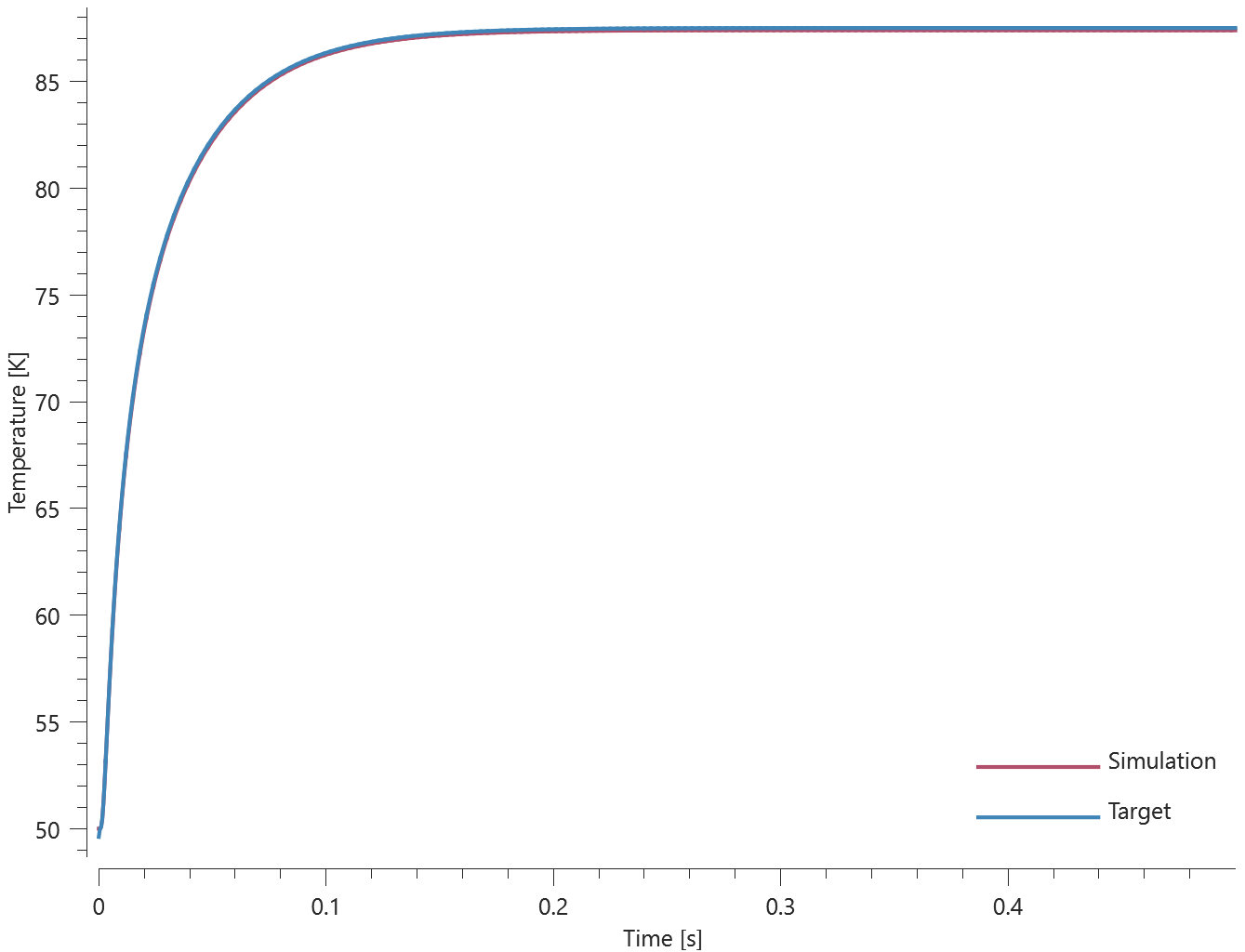
Maximum and average temperature is checked at the sensor.
Tests
This benchmark is associated with 1 tests.
Heat conduction
"Optional title"
tid, $\alpha_T$, $C_p$, $\lambda$, $k$, $T_{ref}$, $\varepsilon$
In this test the thermal conductivity and energy balance functionalities are tested. A metal cylinder impacts a rigid wall and plastic deformations heat up the material. Heat transfer inside the cylinder eventually smears out the thermal energy. The initial kinetic energy, $W_{k}$ , is defined as:
$$ W_{k} = 0.5\cdot m\cdot v^{2} $$
The final temperature at every point inside the cylinder can be calculated as:
$$ T = W_{k}/(mass\cdot C_{p}) = 0.5\cdot m\cdot v^{2} / mass\cdot C_{p} = 0.5\cdot v^{2}/C_{p} = 50 $$
The final temperature in the model is compared to the value from the second equation.
Tests
This benchmark is associated with 1 tests.
*REDISTRIBUTE_MESH_CARTESIAN
Polynomial and exponential mesh redistribution
coid
entype, enid, dir, $c_1$, $c_2$
$x_c$, $y_c$, $z_c$
Tested parameters: coid, entype, enid, dir, $c_1$, $c_2$, $x_c$, $y_c$, $z_c$.
This model tests the command *REDISTRIBUTE_MESH_CARTESIAN. The test consists of a one dimensional beam with length 1 and 10 equally distanced elements. The mesh is redistributed using polynomial and exponential functions.
The polynomial redistribution can be seen in Figure 1 and 2.
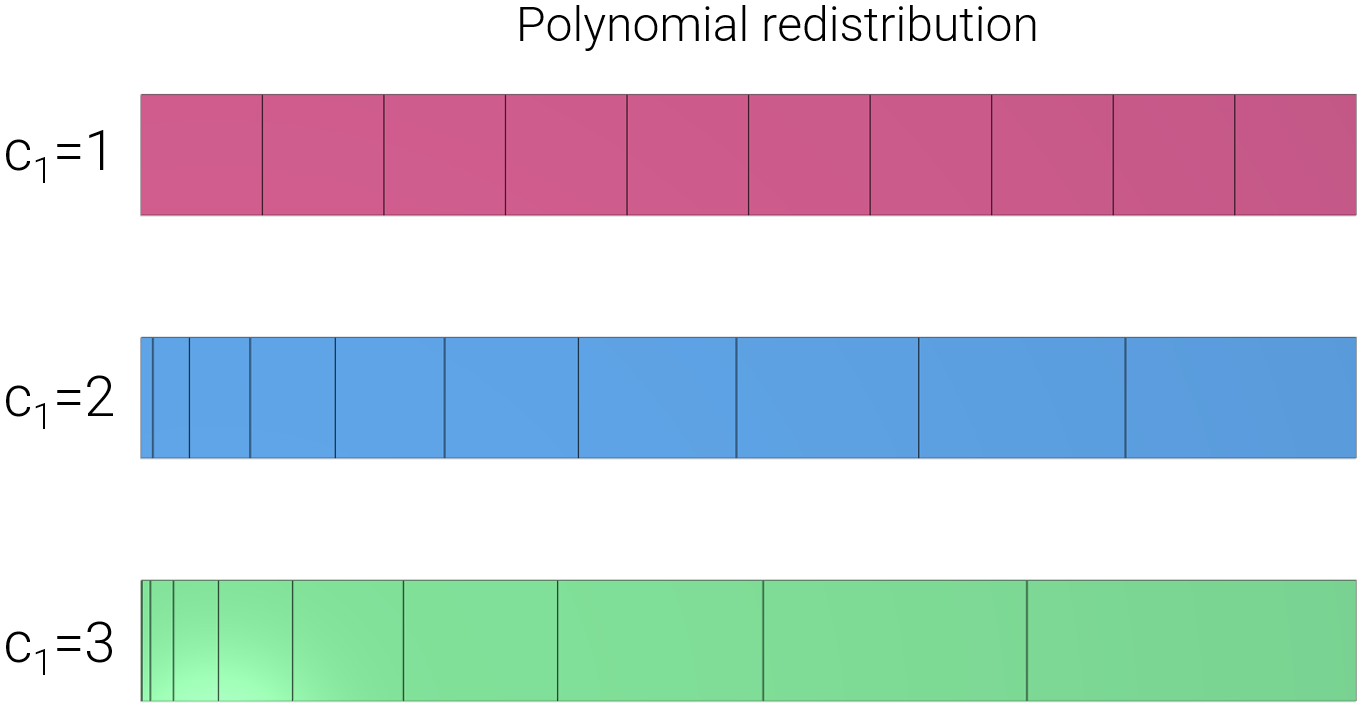
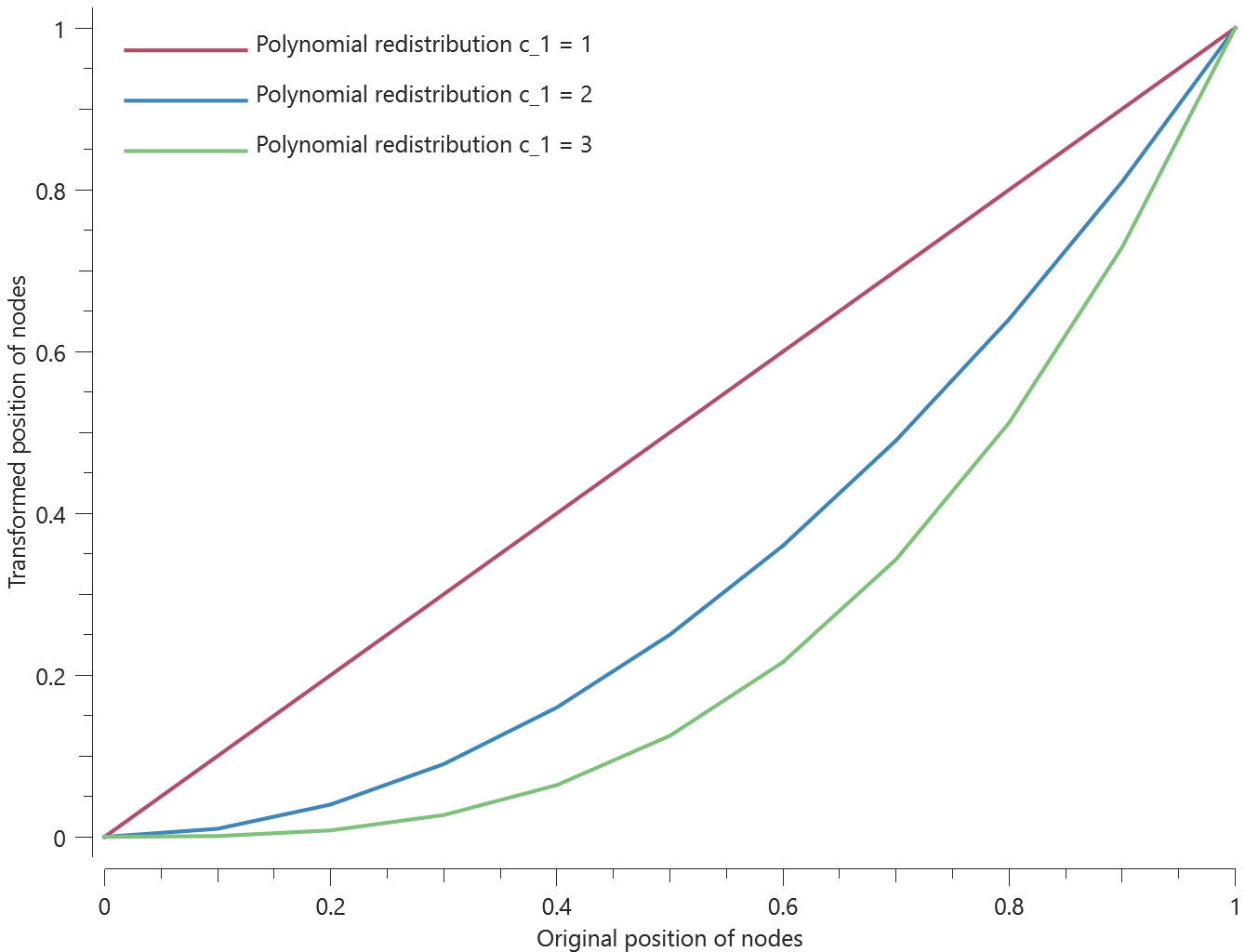
The exponential redistribution can be seen in Figure 3 and 4
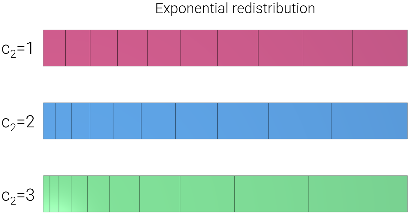
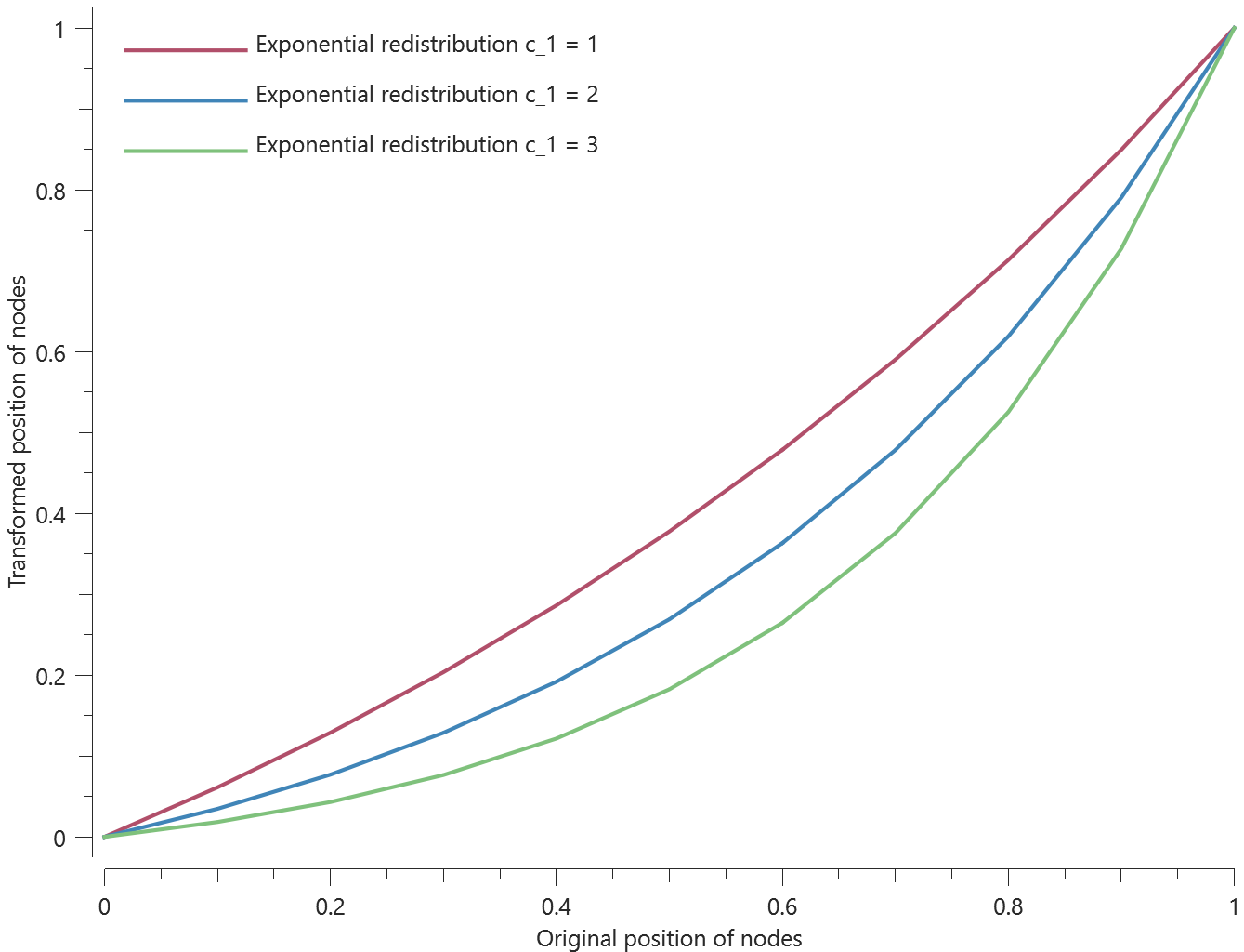
Node positions are checked for version control.
Tests
This benchmark is associated with 1 tests.
*REFINE
Refine pipe
entype, enid, level, gid, thick, $d_{min}$, $\alpha_{max}$, deactivate
This model tests the *REFINE command. The test model is generated using the *COMPONENT_PIPE command. The test model is designed with elements of various dimensions, allowing the $d_{min}$ (minimum element dimension for refinement) feature to be tested. The minimum dimension is set so that only the outer elements are refined. Both the parameter $thick$ (disables refinement in through thickness direction) and the $\alpha_{max}$ (external element face smoothing angle) are active as well. The test model is displayed in Figure 1.
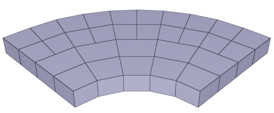
For version control the positioning of two nodes that are affected by the refinement.
Tests
This benchmark is associated with 1 tests.
*REMAP
Elastic rod
"Optional title"
coid
pid$_{from}$, pid$_{to}$, velo, stress, state, defgrad
Tested parameters: coid, $pid_{from}$, $pid_{to}$, velo, stress, state, defrag.
This model tests the command *REMAP. The test consists of 2 steps. A rod of length $0.2 \ m$ is elastically elongated by 10% in uniaxial tension to a total length of $0.22 \ m$. Once fully elongated it is released and returns to its original shape. See Figure 1
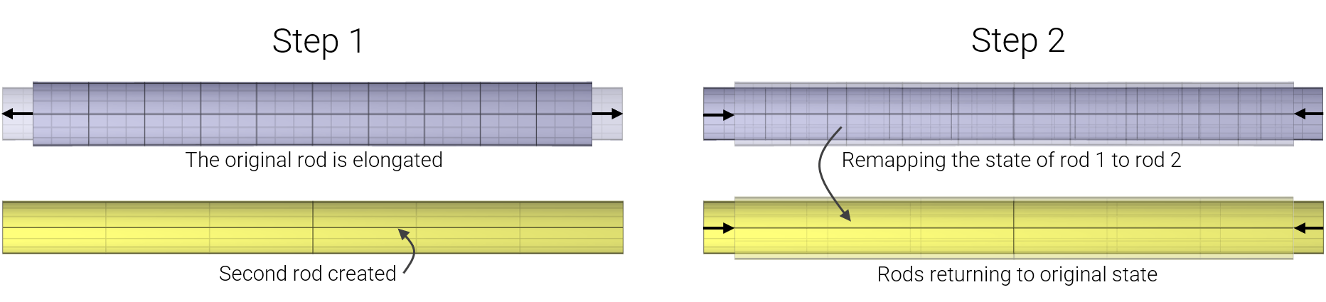
In step 1, the rod is elongated and the simulation is terminated. A new rod with same dimension and position of the elongated rod is created but with different mesh size.
In step 2, the state of the deformed rod is mapped to the undeformed rod with the command *REMAP. Since the prescribed motion has been removed from the model and since the rods are in an identical state due to mapping, both rods should return to the original undeformed state.
Target strain at full elongation: $$ \varepsilon_{engineering} = \frac{l-L}{L} = \frac{0.22-0.2}{0.2} = 0.1 $$ $$ \varepsilon_{true} = ln(1+\varepsilon_{engineering}) = ln(1+0.1) = 0.09531 $$
Total length and strain generated from the elongation simulated in step 1 is measured with sensors. See Figure 2.
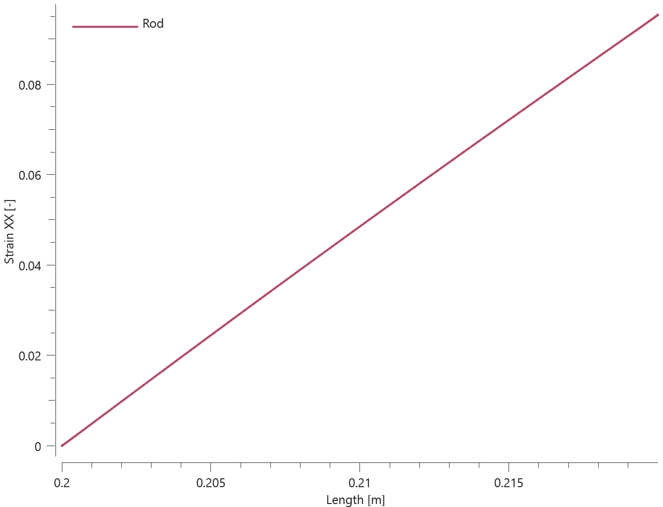
The elongated and remapped rod going back to original dimension simulated in step 2 is illustrated in Figure 3. Damping is applied.
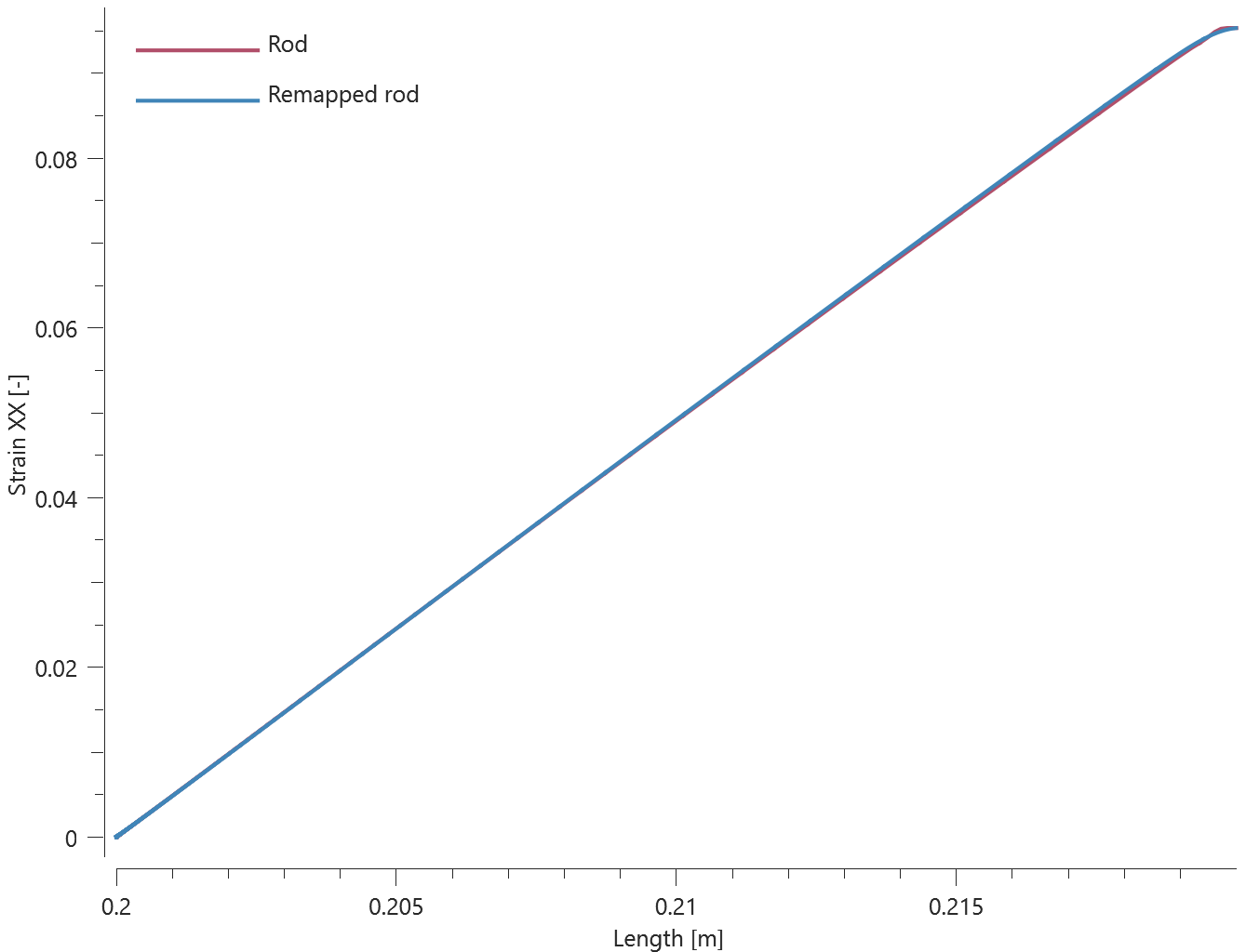
The total length, effective stress and true strain in undeformed and deformed state for both rods is checked for version control.
Tests
This benchmark is associated with 2 tests.
*RIGID_BODY_ADD_NODES
Rigid box guiding beam
"Optional title"
coid
pid, entype, enid
Tested parameters: coid, pid, entype, enid.
This model tests the functionality of the command *RIGID_BODY_ADD_NODES. The test model consists of a cantilever beam and a rigid box. A displacement of $1 \ mm$ in the negative Z-direction is prescribed to the rigid box, which is connected to the nodes at the free end of the beam with the command *RIGID_BODY_ADD_NODES.
To test the functionality of the command, three identical test setups are created, using different entity types to add the deformable nodes to the rigid bodies. The entity types tested are:
- Node, N
- Node set, NS
- Geometry, G
The test setup is displayed in Figure 1.
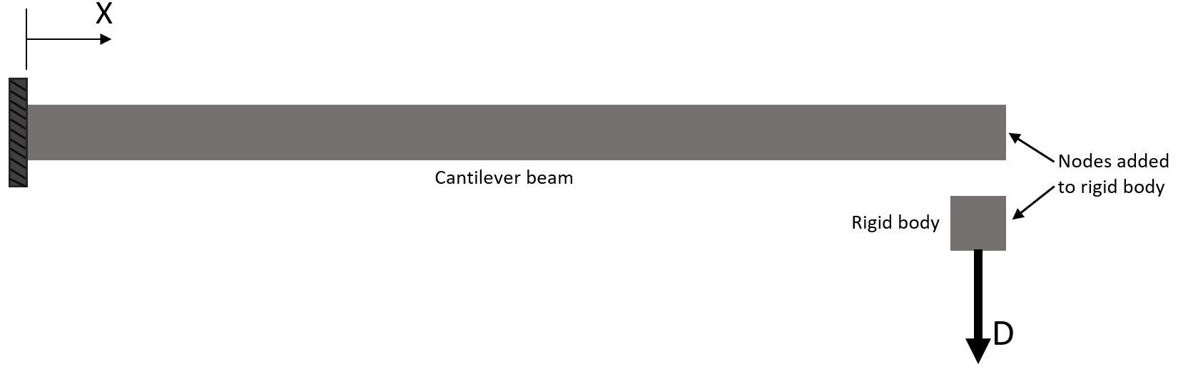
Sensors are placed at the free end of the beams to measure the tip displacement.
Targets:
Maximum deflection for all beams = $1 \ mm$.
Tests
This benchmark is associated with 1 tests.
*RIGID_BODY_DAMPING
Damping between moving and constrained body
pid${}_1$, pid${}_2$, $C$, $t_{beg}$, $t_{end}$
This tests the *RIGID_BODY_DAMPING command. One rigid body is constrained from all motion while another rigid body is given an initial velocity towards the other. A damping force is defined between the bodies, and final displacement of the moving body is checked for version control.
Tests
This benchmark is associated with 1 tests.
*RIGID_BODY_INERTIA
Rolling cylinders
pid, $m$, $x_c$, $y_c$, $z_c$, $I_{11}$, $I_{22}$, $I_{33}$
$I_{12}$, $I_{23}$, $I_{31}$
Tested parameters: pid, $m$, $x_c$, $y_c$, $z_c$, $I_{11}$, $I_{22}$, $I_{33}$, $I_{12}$, $I_{23}$, $I_{31}$.
The model tests the *RIGID_BODY_INERTIA command. Five rigid bodies with the geometry of solid cylinders with equivalent dimensions and masses are rolling downwards an inclined plane due to gravity. With the command *RIGID_BODY_INERTIA one can define mass, center of gravity & moment of inertia. The cylinders that are assigned a higher moment of inertia will go down the plane slower, since more potential energy is needed to be converted into kinetic energy.
The test setup is displayed in Figure 1.
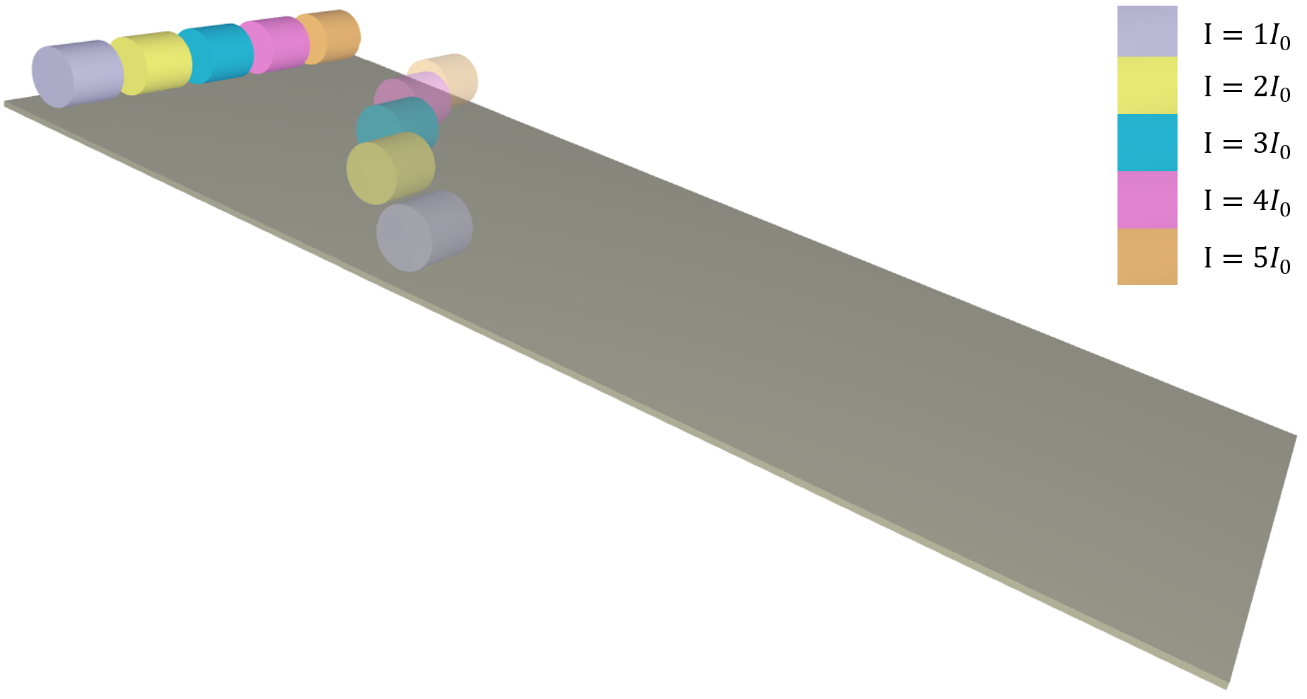
The friction coefficient is set to a high value so that no slipping is allowed. Also, dissipative forces are being ignored. For this test setup, we get conservation of energy:
$$ mgh = \dfrac{1}{2} mv^2 + \dfrac{1}{2} I \left( \dfrac{v}{r}\right)^2 $$
Test parameters:
| Cylinder radius: | $r = 0.05 \ m$ |
| Cylinder height: | $h = 0.1 \ m$ |
| Cylinder Mass: | $m = 6.12552 \ kg$ |
| Inclination of plane: | $\alpha = 14.036°$ |
| Gravity: | $g =9.82 \ m/s^{2}$ |
| Dimensionless constant MOI: | $k = 1/2$ |
| Moment of inertia multiplier: | $q = 1,2,3,4,5$ |
| Moment of inertia cylinder: | $I = q \cdot k \cdot m{r}^2$ |
Kinetic energy vs. time is displayed in Figure 2 together with target curves from a verification script.
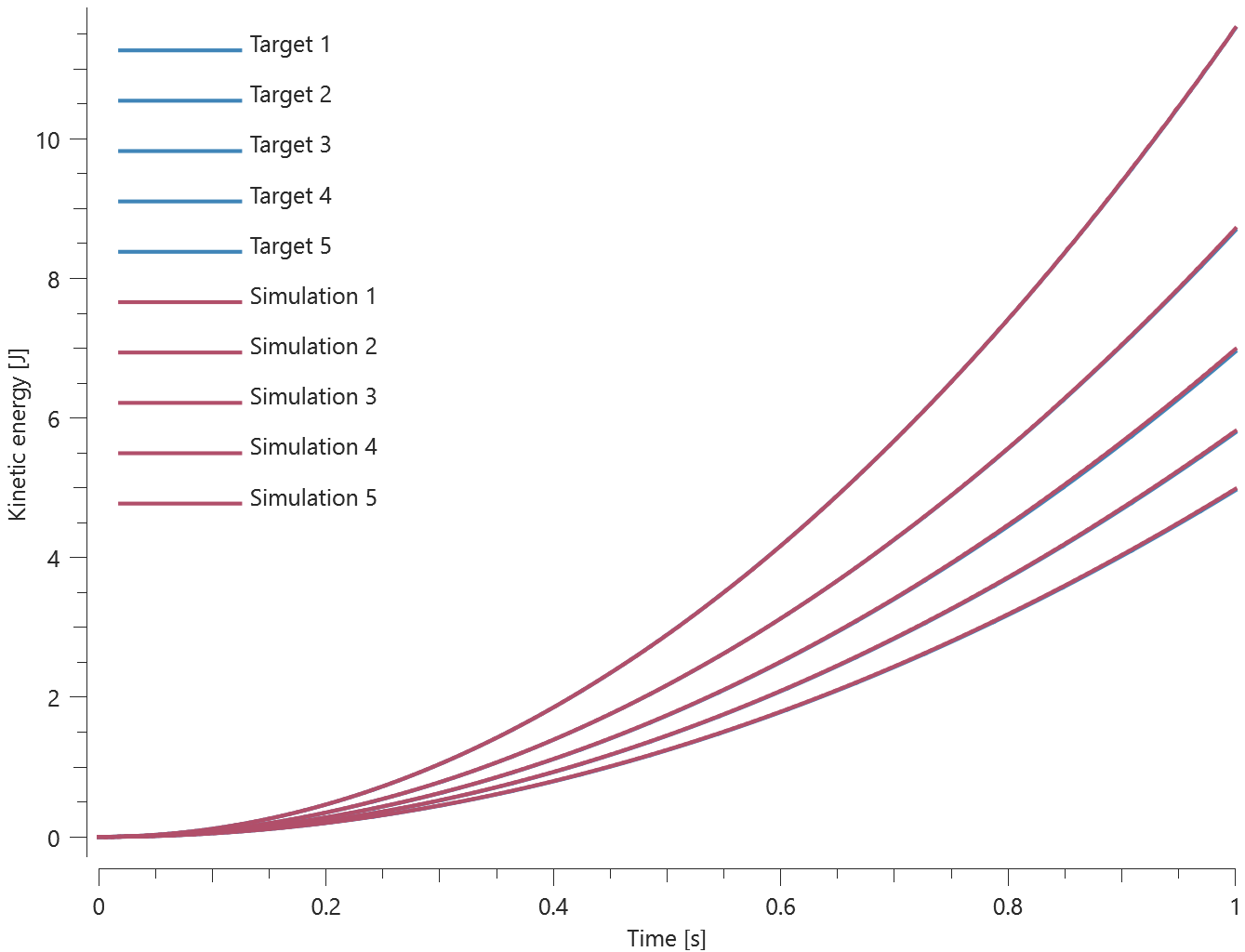
Last values of kinetic energy is checked for version control.
Accepted error: (+/-) 1%
Tests
This benchmark is associated with 1 tests.
*RIGID_BODY_JOINT
Ability to handle rotations
"Optional title"
coid
entype${}_1$, enid${}_1$, entype${}_2$, enid${}_2$, bc${}_{tr}$, bc${}_{rot}$, csysid${}_1$, csysid${}_2$
$rx-$, $rx+$, $ry-$, $ry+$, $rz-$, $rz+$, $gap$, $\xi$, $pfac$
cid${}_{Tx}$, cid${}_{Ty}$, cid${}_{Tz}$, $T^f_x$, $T^f_y$, $T^f_z$, cid${}_{Fx}$, cid${}_{Fy}$, cid${}_{Fz}$
This tests the *RIGID_BODY_JOINT command. Specifically, it tests the ability of a rigid body joint to correctly handle rotations. The model contains two rigid bodies, a cylindrical shaft and a thin-walled pipe, as seen in Figure 1. We effectively have a glide bearing, where the thin-walled pipe is mounted on and spins around the cylindrical shaft. The interaction between the shaft and the pipe is handled by a rigid body joint.
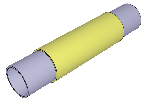
The joint allows for free rotations in the axial direction. All other local degrees of freedom are constrained. At time zero, the shaft is oriented with its axial direction along the global X-axis. The pipe spins with $1000 \ rad/s$ around the shaft and the spin vector at time zero is ($1000, 0, 0$). The shaft is slowly turned 90° (*BC_MOTION) and at termination time it has shifted its axial orientation from ($1, 0, 0$) to ($0, 1, 0$). At the same time the spin vector of the pipe should have changed from ($1000, 0, 0$) to ($0, 1000, 0$).
For version control, the spin of the cylinder is checked in "rigid.out".
Tests
This benchmark is associated with 1 tests.
Conservation of energy
"Optional title"
coid
entype${}_1$, enid${}_1$, entype${}_2$, enid${}_2$, bc${}_{tr}$, bc${}_{rot}$, csysid${}_1$, csysid${}_2$
$rx-$, $rx+$, $ry-$, $ry+$, $rz-$, $rz+$, $gap$, $\xi$, $pfac$
cid${}_{Tx}$, cid${}_{Ty}$, cid${}_{Tz}$, $T^f_x$, $T^f_y$, $T^f_z$, cid${}_{Fx}$, cid${}_{Fy}$, cid${}_{Fz}$
This tests the *RIGID_BODY_JOINT command. Two rigid spheres are connected with a joint (fully constrained in translation and rotation). The spheres have an initial velocity in the Z-direction. One of the spheres impacts a rigid plane and reverses its velocity. As a system, it goes from translation to nearly pure spin.
| Sphere radius: | $r = 0.03 \ m$ |
| Distance between spheres (center to center): | $D = 0.2 \ m$ |
| Mass density: | $\rho = 1000 \ kg/m^{3}$ |
| Sphere mass: | $m =\rho \cdot 4\pi r^{3}/3$ |
| Moment of inertia of system: | $I = m\left( 0.8r^2 + 0.5D^2\right)$ |
| Initial translational velocity: | $v_0 = -1 \ m/s$ |
| Kinetic energy of system: | $E_k = 2 \cdot m{v_0}^2$ |
After impact very close to 100% of the energy is transformed into spin. That is:
$$ E_k = 0.5\cdot I\cdot \boldsymbol{\omega}^2 $$
$$ {v_0}^2 = \left( \dfrac{2}{5}r^2 + \left( \dfrac{D}{2}\right) ^2 \right) \cdot \omega^2 $$
$$ \omega = 9.82 rad/s $$
This spin can be found in "rigid.out" (Y-component) and it should be the same for both rigid bodies.
Tests
This benchmark is associated with 1 tests.
Torsional spring
"Optional title"
coid
entype${}_1$, enid${}_1$, entype${}_2$, enid${}_2$, bc${}_{tr}$, bc${}_{rot}$, csysid${}_1$, csysid${}_2$
$rx-$, $rx+$, $ry-$, $ry+$, $rz-$, $rz+$, $gap$, $\xi$, $pfac$
cid${}_{Tx}$, cid${}_{Ty}$, cid${}_{Tz}$, $T^f_x$, $T^f_y$, $T^f_z$, cid${}_{Fx}$, cid${}_{Fy}$, cid${}_{Fz}$
This test verifies the functionality of *RIGID_BODY_JOINT. Two bodies are connected with a rigid body joint. The joint is located at the center of the box, see Figure 1. The joint is equipped with a linear torsional spring. The simulation is split into two stages:
Stage 1: The box is rotated $\pi$/2 rad around the Z-axis while the sphere is held fixed in space. This builds up a torque in the spring.
Stage 2: The box is held completely fixed while the sphere is released. The torque from Stage 1 will accelerate the sphere and it will start rotate around the joint.
The rotation of the sphere at termination is checked and verified against an analytical solution.
Tests
This benchmark is associated with 1 tests.
*RIGID_BODY_MERGE
Test 1
"Optional title"
setid
Two rigid spheres are connected with *RIGID_BODY_MERGE. The spheres have an initial velocity in the Z-direction. One of the spheres impacts a rigid plane and reverses its velocity. As a system, it goes from translation to nearly pure spin.
| Sphere radius: | $r = 0.03 \ m$ |
| Distance between spheres (center to center): | $D = 0.2 \ m$ |
| Mass density: | $\rho = 1000 \ kg/m^{3}$ |
| Sphere mass: | $m =\rho \cdot 4\pi r^{3}/3$ |
| Moment of inertia of system: | $I = m\left( 0.8r^2 + 0.5D^2\right)$ |
| Initial translational velocity: | $v_0 = -1 \ m/s$ |
| Kinetic energy of system: | $E_k = 2 \cdot m{v_0}^2$ |
After impact very close to 100% of the energy is transformed into spin. That is:
$$ E_k = 0.5\cdot I\cdot {\omega}^2 $$
$$ {v_0}^2 = \left( \dfrac{2}{5}r^2 + \left( \dfrac{D}{2}\right) ^2 \right) \cdot {\omega}^2 $$
$$ {\omega} = {9.82} \ rad/s $$
This spin can be found in "rigid.out" (Y-component) and it should be the same for both rigid bodies.
Tests
This benchmark is associated with 1 tests.
*RIGID_BODY_UPDATE
Curvlinear update
type
Tested parameters: type.
This test is created in combination with the test "*RIGID_BODY_UPDATE - Linear update". The test setup is modelled the same, but curvlinear update is used in this test instead.
Targets:
- Linear update - Rigid cylinder radius increase (see the test "*RIGID_BODY_UPDATE - Linear update")
- Curvlinear update - The rigid cylinder radius do not change
First, average and last values of sensor radius is checked for version control.
Tests
This benchmark is associated with 1 tests.
Linear update
type
Tested parameters: type.
This test is created in combination with the test "*RIGID_BODY_UPDATE - Curvlinear update".
The model tests the *RIGID_BODY_UPDATE command. The test consists of two cylinders, one is rigid and the other deformable. The cylinders are next to one another and duplicated nodes are merged.
The free end of the deformable cylinder is fixed and the rigid cylinder is rotating around its central axis, which creates a torsion. See Figure 1.

By default (in order to conserve energy) rigid body nodes follow incremental linear paths during time integration, when interacting with deformable bodies. This can lead to significant geometrical errors if both time step size and the rigid body rotations are large. See Figure 2.
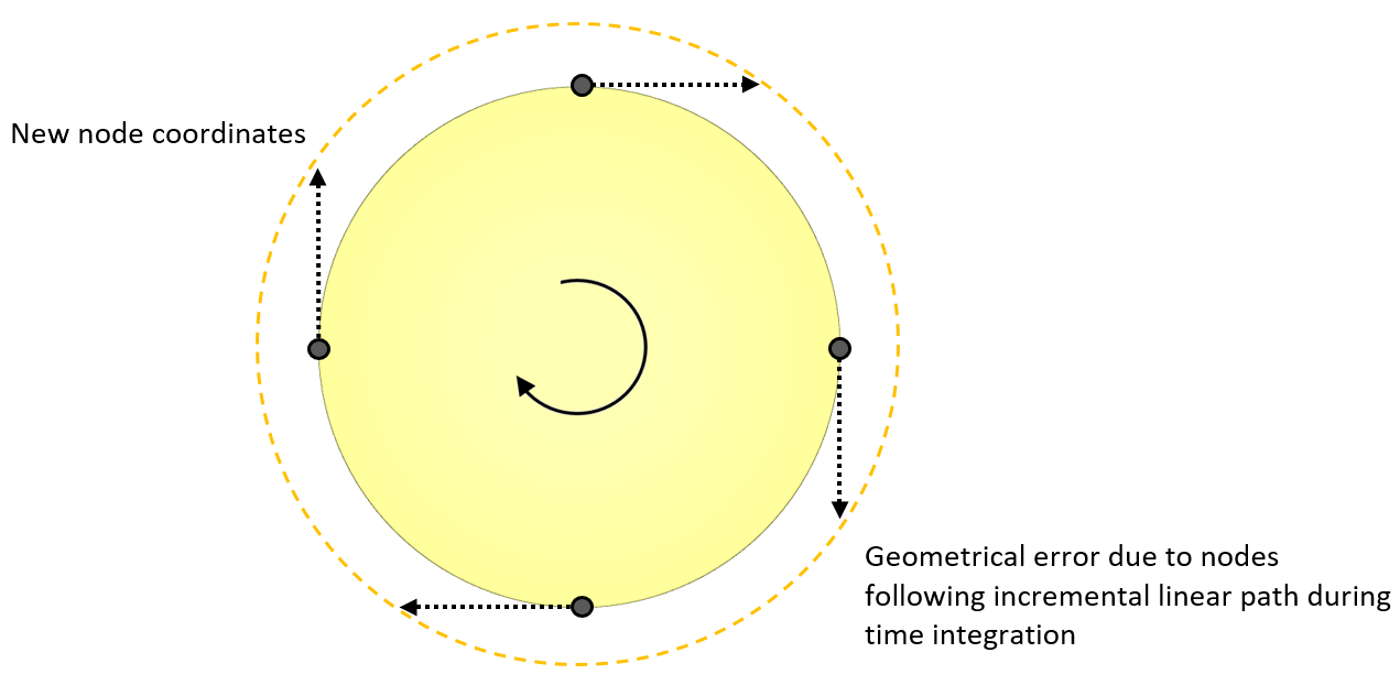
An output sensor that measure radius is placed at the center of the rigid cylinder to measure if the cylinder radius is expanding during the test.
Targets:
- Linear update - Rigid cylinder radius increase
- Curvlinear update - The rigid cylinder radius do not change (see the test "*RIGID_BODY_UPDATE - Curvlinear update")
First, average and last values of sensor radius is checked for version control.
Tests
This benchmark is associated with 1 tests.
*SCRIPT_PYTHON
Control time and output
filename
The model tests the *SCRIPT_PYTHON command. The test consists of discrete particles that are falling down towards a flat rigid plate. Coming in contact with the plate, after some time the particles will stop moving and hence looses kinetic energy. See Figure 1.
To avoid uneccesary simulation time a python script is used to control the termination time with a function that evaluates time, total kinetic energy of the model and a target value for the kinetic energy. Also the output interval for ASCII data, $\Delta t_{ascii}$, is being controlled with a python script.
Target:
- If the kinetic energy goes below the target value the simulation should end.
Tests
This benchmark is associated with 1 tests.
*SCRIPT_PYTHON_CODE
Function
filename
code
This model tests the command *SCRIPT_PYTHON_CODE. The command is used to load embedded python code directly from the input file which can be used in FUNCTION. The test consists of two components that are set in motion instructed by python code. An embedded python script returns a value at a given time for the function defining the prescribed motion of the first component. For reference an equivalent instruction is assigned to the second component with *SCRIPT_PYTHON.
Targets:
- *SCRIPT_PYTHON and *SCRIPT_PYTHON_CODE should give the same result.
Tests
This benchmark is associated with 1 tests.
*SET_ELEMENT
Multi-functionality test
"Optional title"
setid
eid${}_1$, ..., eid${}_8$
.
eid${}_{\mathrm{M}}$, ..., eid${}_{\mathrm{N}}$
Tested parameters: setid, eid${}_1$ - eid${}_8$.
This model tests that *SET_ELEMENT is compatible in combination with the following commands.
Tested combinations:
- *SET_ELEMENT in *ACTIVATE_ELEMENTS
- *SET_ELEMENT in *OUTPUT_ELEMENT
The test setup is straightforward.
- Components, (two when needed) are created for each test combination.
- A simple action is implemented for each combination.
- Afterwards it is verified wether the action has been conducted or not.
Tests
This benchmark is associated with 1 tests.
*SET_FACE
Multi-functionality test
"Optional title"
setid
nid${}_{11}$, nid${}_{12}$, nid${}_{13}$, nid${}_{14}$
.
nid${}_{\mathrm{N1}}$, nid${}_{\mathrm{N2}}$, nid${}_{\mathrm{N3}}$, nid${}_{\mathrm{N4}}$
Tested parameters: setid, $nid_{11}$ - $nid_{14}$, $nid_{N1}$ - $nid_{N4}$.
This model tests that *SET_FACE is compatible in combination with the following commands.
Tested combinations:
- *SET_FACE in *LOAD_FORCE
- *SET_FACE in *LOAD_PRESSURE
- *SET_FACE in *LOAD_SHEAR
- *SET_FACE in *LOAD_THERMAL_SURFACE
- *SET_FACE in *LOAD_THERMAL_RADIATION
The test setup is straightforward.
- Components, (two when needed) are created for each test combination.
- A simple action is implemented for each combination.
- Afterwards it is verified wether the action has been conducted or not.
Tests
This benchmark is associated with 1 tests.
*SET_GEOMETRY
Multi-functionality test
"Optional title"
setid
gid${}_1$, ..., gid${}_8$
.
gid${}_{\mathrm{M}}$, ..., gid${}_{\mathrm{N}}$
Tested parameters: setid, gid${}_1$ - gid${}_8$, gid${}_M$ - gid${}_N$.
This model tests that *SET_GEOMETRY is compatible in combination with the following commands.
Tested combinations:
- *SET_GEOMETRY in *ACTIVATE_ELEMENTS
- *SET_GEOMETRY in *BC_MOTION
- *SET_GEOMETRY in *LOAD_PRESSURE
- *SET_GEOMETRY in *LOAD_THERMAL_SURFACE
- *SET_GEOMETRY in *RIGID_BODY_ADD_NODES
- *SET_GEOMETRY in *TRANSFORM_MESH_CARTESIAN
- *SET_GEOMETRY in *TRANSFORM_MESH_CYLINDRICAL
- *SET_GEOMETRY in *LOAD_THERMAL_RADIATION
The test setup is straightforward.
- Components, (two when needed) are created for each test combination.
- A simple action is implemented for each combination.
- Afterwards it is verified wether the action has been conducted or not.
Tests
This benchmark is associated with 1 tests.
Pressure with geometry set
"Optional title"
setid
gid${}_1$, ..., gid${}_8$
.
gid${}_{\mathrm{M}}$, ..., gid${}_{\mathrm{N}}$
Tested parameters: setid, gid${}_1$ - gid${}_8$, gid${}_M$ - gid${}_N$.
This model tests the *SET_GEOMETRY command. The test consists of a pressure load on a surface defined with a geometrical set. There are four geometries. See Figure 1.
- Geometry 1 marks all faces on the top surface of the plate.
- Geometry 2 is a box. Referring to -2 means that all faces inside the box are removed from the face list.
- Geometry 3 adds faces inside a cylinder.
- Geometry 4 removes faces inside the box, by referring to it as -4.
A load pressure is applied to the model, defined with the geometrical set. Four sensors are placed at given positions to measure the surface pressure, See Figure 2.
Targets:
- Sensor 1: Contact/applied pressure = 0 Pa
- Sensor 2: Contact/applied pressure = 1e5 Pa
- Sensor 3: Contact/applied pressure = 0 Pa
- Sensor 4: Contact/applied pressure = 1e5 Pa
Tests
This benchmark is associated with 1 tests.
*SET_NODE
Multi-functionality test
"Optional title"
setid
nid${}_1$, ..., nid${}_8$
.
nid${}_{\mathrm{M}}$, ..., nid${}_{\mathrm{N}}$
Tested parameters: setid, nid${}_1$ - nid${}_8$, nid${}_M$ - nid${}_N$.
This model tests that *SET_NODE is compatible in combination with the following commands.
Tested combinations:
- *SET_NODE in *BC_MOTION
- *SET_NODE in *CONNECTOR_RIGID
- *SET_NODE in *INITIAL_VELOCITY
- *SET_NODE in *LOAD_CENTRIFUGAL
- *SET_NODE in *LOAD_DAMPING
- *SET_NODE in *LOAD_FORCE
- *SET_NODE in *MERGE
- *SET_NODE in *OUTPUT_NODE
- *SET_NODE in *OUTPUT_USER_COLLECTION
- *SET_NODE in *RIGID_BODY_ADD_NODES
- *SET_NODE in *SMOOTH_MESH
The test setup is straightforward.
- Components, (two when needed) are created for each test combination.
- A simple action is implemented for each combination.
- Afterwards it is verified wether the action has been conducted or not.
Tests
This benchmark is associated with 1 tests.
*SMOOTH_MESH
Rigid plate
"Optional title"
entype, enid, $\alpha_{\mathrm{max}}$, internal, gid
csysid
This model tests the *SMOOTH_MESH command. The command is applied to a rigid plate with a hole. The hole is at the center and has the shape of a hexagon, see Figure 1. The coordinates of a node on the edge of the hole is checked for version control.
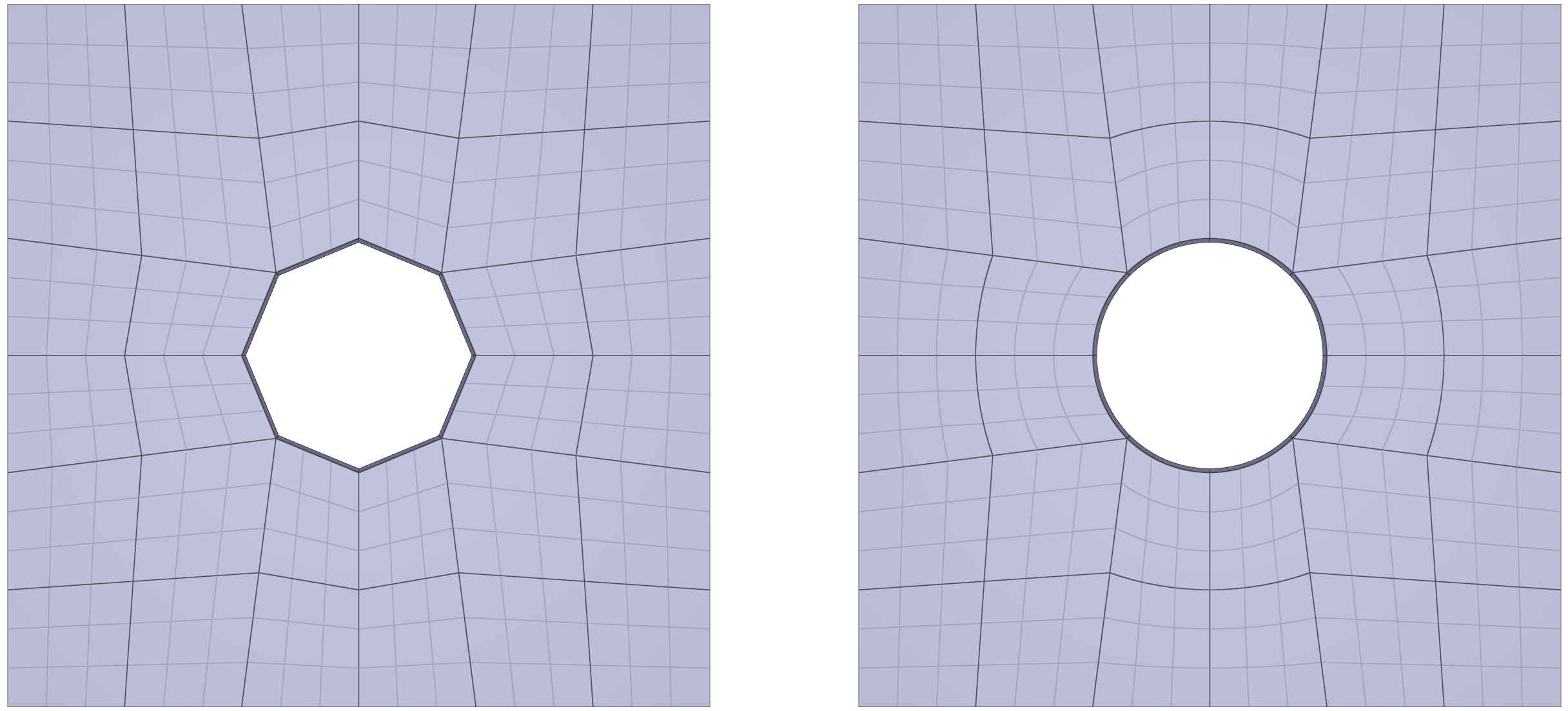
Tests
This benchmark is associated with 1 tests.
csysid
"Optional title"
entype, enid, $\alpha_{\mathrm{max}}$, internal, gid
csysid
Tested parameters: csysid.
This model tests the command *SMOOTH_MESH. Three identical cones are created. *SMOOTH_MESH with a smoothing angle of 45° is used for the second and third cone. To avoid mesh smoothing node displacements in the axial direction, the parameter $csysid$ is used for the third cone. The axial direction is defined with a cylindrical coordinate system. The test setup is displayed in Figure 1.
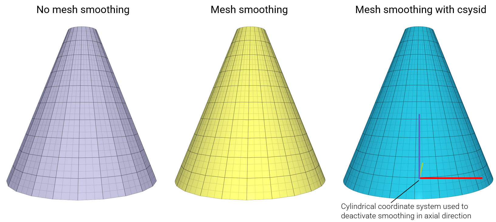
Aim: Turn off mesh smoothing in specific direction (coordinate system based).
Target:
- node.out -> z-coordinate = 0.5 (max error 1.0e-6)
Tests
This benchmark is associated with 1 tests.
*SMS
Selective Mass Scaling
"Optional title"
entype, enid, $sf$
This tests the *SMS command. Selective mass scaling is a method to increase the critical time step size by modifying the mass matrix (non-diagonal) while at the same time leaving the rigid body translational behavior unaffected. It is computationally expensive as a linear equation system needs to be solved every time step. The benefit is less non-physical inertia effects than with regular mass scaling. The model is a steel strip impacting a rigid, fixed cylinder as seen in Figure 1.
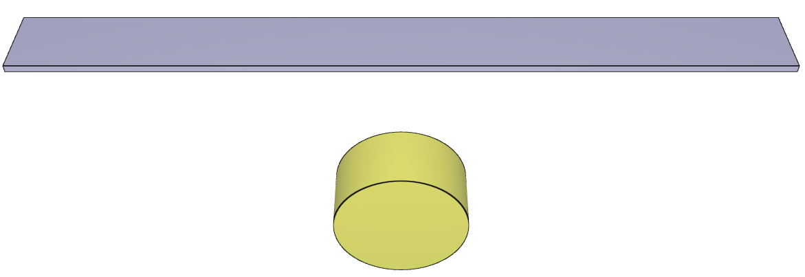
Three simulations using this model is carried out (a forth one is done in the *SMS_CLUSTER benchmark). Firstly, no mass scaling is allowed. This gives the most accurate result, the drawback being a longer simulation time. Secondly, regular mass scaling is applied using the *TIME command. Extra mass is added to the nodes of the model. It is computationally fast, but will inevitably affect the dynamic behavior of the structure. Lastly, the *SMS command is activated. The results are shown in Table 1.
| Simulation | Peek displacement [m] | Normalized computational time [-] |
|---|---|---|
| No mass scaling | 0.050 | 1 |
| Regular mass scaling | 0.063 | 0.44 |
| Selective mass scaling | 0.048 | 0.77 |
For version control, the peek displacement of a node at the tip of the strip is checked.
Tests
This benchmark is associated with 3 tests.
*SUBDIVIDE_PART_THICKNESS
Absolute face sheet thickness
"Optional title"
coid
pid, tid, $x_f$, $y_f$, $z_f$, absolute
Tested parameters: coid, pid, tid, $x_f$, $y_f$, $z_f$, absolute.
This model tests the command *SUBDIVIDE_PART_THICKNESS. A solid component with one element in thickness direction and a varying thickness ranging from $6 \ mm$ to $10 \ mm$ is subdivided into a sandwich structure with two face layers and a core. See Figure 1.
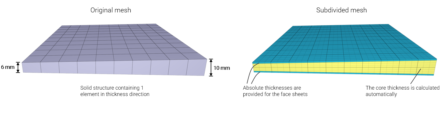
With the absolute thickness option flag (absolute=1), the face sheets are given a fixed thickness while the core a varying thickness. Absolute thicknesses of $0.8 \ mm$ are specified for the face layers and 0 for the core, which means that the core thickness is automatically determined from the original part thickness minus face sheet thicknesses.
The volume of the subdivided parts is checked for version control.
$$V_{core} = 1 \cdot 1 \cdot (0.084+0.044)/2 = 0.064 \ m^2 $$ $$ V_{Face sheets} = 2 \cdot (0.008 \cdot 1 \cdot 1) = 0.016 \ m^2 $$
Tests
This benchmark is associated with 1 tests.
*TIME
Maximum allowed mass scaling factor
$t_{term}$, $sf_{\Delta t}$, $\Delta t_{\mathrm{min}}$, $\Delta t_{\mathrm{max}}$, $ms_{\mathrm{max}}$, $t_{start}$
Maximum allowed mass scaling factor is verified in this test.
Tested parameters: $ms_{\mathrm{max}}$ and $\Delta t_{\mathrm{min}}$.
A minimum allowed time step size significantly larger than the default time step size is defined in the model. A maximum allowed mass scaling factor is also defined. With this configuration, the time step is scaled, but only to such an extent that the mass scaling factor does not exceed the maximum allowed mass scaling factor.
Time step size and mass scaling factor are checked for version control.
Tests
This benchmark is associated with 1 tests.
Maximum and minimum time step size
$t_{term}$, $sf_{\Delta t}$, $\Delta t_{\mathrm{min}}$, $\Delta t_{\mathrm{max}}$, $ms_{\mathrm{max}}$, $t_{start}$
Maximum and minimum time step size are verified in this test.
Tested parameters: $\Delta t_{\mathrm{min}}$ and $\Delta t_{\mathrm{max}}$.
A maximum allowed time step size is imposed in one model, and a minimum in another model.
The time step sizes are checked for version control.
Tests
This benchmark is associated with 2 tests.
Termination time and time step size
$t_{term}$, $sf_{\Delta t}$, $\Delta t_{\mathrm{min}}$, $\Delta t_{\mathrm{max}}$, $ms_{\mathrm{max}}$, $t_{start}$
Termination time, default time step size and scaled time step size are verified in this test.
Tested parameters: $t_{term}$ and $sf_{\Delta t}$.
Two models are used. In the first model, the termination time and default time step size is checked for version control. In the second model, a scale factor of 0.5 is used for the time step, meaning that the time step size in this model should be $0.5/0.9 \cdot \Delta t_{default}$, since the default scale factor is 0.9.
All solid element types are tested. Termination time and time step size are checked for version control.
Tests
This benchmark is associated with 18 tests.
*TRANSFORM_MESH_CARTESIAN
Rigid elements
"Optional title"
coid, entype, enid, csysid, fid${}_1$, fid${}_2$, fid${}_3$
This model tests the *TRANSFORM_MESH_CARTESIAN command. A single rigid element is created using the *COMPONENT_BOX command with opposite nodes at ($0,0,0$) and ($1,1,1$). This mesh is then translated along all axis by a constant of 10. The resulting positioning of the box should therefore give node coordinates ($10, 10, 10$) and ($11, 11, 11$). This is checked for version control.
Tests
This benchmark is associated with 1 tests.
*TRANSFORM_MESH_CYLINDRICAL
Rigid elements
"Optional title"
coid, entype, enid, csysid, fid${}_1$, fid${}_2$, fid${}_3$, fid${}_4$
This model tests the *TRANSFORM_MESH_CYLINDRICAL command. A single rigid element is created using the *COMPONENT_BOX command with opposite nodes at ($0,0,0$) and ($1,1,1$). This mesh is then translated 1 unit along the axial direction and 45° along the tangential direction. The resulting positioning of the box should therefore give node coordinates ($0,0,1$) and ($0,\sqrt 2,2$). This is checked for version control.
Tests
This benchmark is associated with 1 tests.
*TRIM
Trim elements
entype, enid, nid${}_{seed}$, $t_{trim}$, $\hat{x}$, $\hat{y}$, $\hat{z}$
$x_1$, $y_1$, $z_1$
.
$x_n$, $y_n$, $z_n$
This model tests the command *TRIM. A trim line is defined on a metal sheet, cutting it in half. A seed node marks the material to keep after trimming.
It is checked that the correct side is kept after the trimming operation.
Tests
This benchmark is associated with 1 tests.
*UNIT_SYSTEM
Conversion between unit systems
units, temperature
The following quantities are convertet from all to all unit systems:
| mass | coordinate | length | displacement |
| area | volume | time | stress |
| pressure | energy | power | acceleration |
| velocity | temperature | force | torque |
| moment | impulse | momentum | density |
| viscosity | srate | impint | cstiff |
| sstiff | sdstiff |
The following unit systems are investigated:
| SI | MMTONS |
| CMGUS | IPS |
| MMKGMS | CMGS |
| MMGMS | MMMGMS |
In the example below, parameter $m$, $l$ and $t$ are converted from SI to MMTONS.
*UNIT_SYSTEM
MMTONS
~convert_from_SI
*PARAMETER
m  = 1,  "Mass in SI",      0,  Mass
l  = 2,  "Length in SI",    0,  Length
t  = 3,  "Time in SI",      0,  Time
~end_convert
Tests
This benchmark is associated with 8 tests.
Mass, time, length of all unit systems
units, temperature
A cube with side length of $0.1 \ m$ and a mass of $0.78 \ kg$ is moving in the X-direction with a constant velocity of $100.0 \ m/s$ during $0.01 \ s$. All the available unit systems are tested (SI, MMTONS, CMGUS, IPS, MMKGMS, CMGS MMGMS and MMMGMS). The volume, mass, velocity and time step size is checked for version control.
Tests
This benchmark is associated with 8 tests.
*VELOCITY_CAP
AIR and HE
$v_{max}^{N}$, $v_{max}^{DP1}$, $v_{max}^{DP2}$, $v_{max}^{CFD}$
Tested parameters: $v_{max}^{DP2}$.
This model tests maximum allowed discrete particle high explosive and discrete particle air velocities with the command *VELOCITY_CAP. A spherical discrete particle HE subdomain of TNT is detonated which generates extreme velocities. Also, a spherical discrete particle AIR subdomain is expanding in the global domain. An upper limit of $500 \ m/s$ is set to $v_{max}^{DP2}$ which prevents the AIR and HE particles reaching higher levels of velocity. See Figure 1.
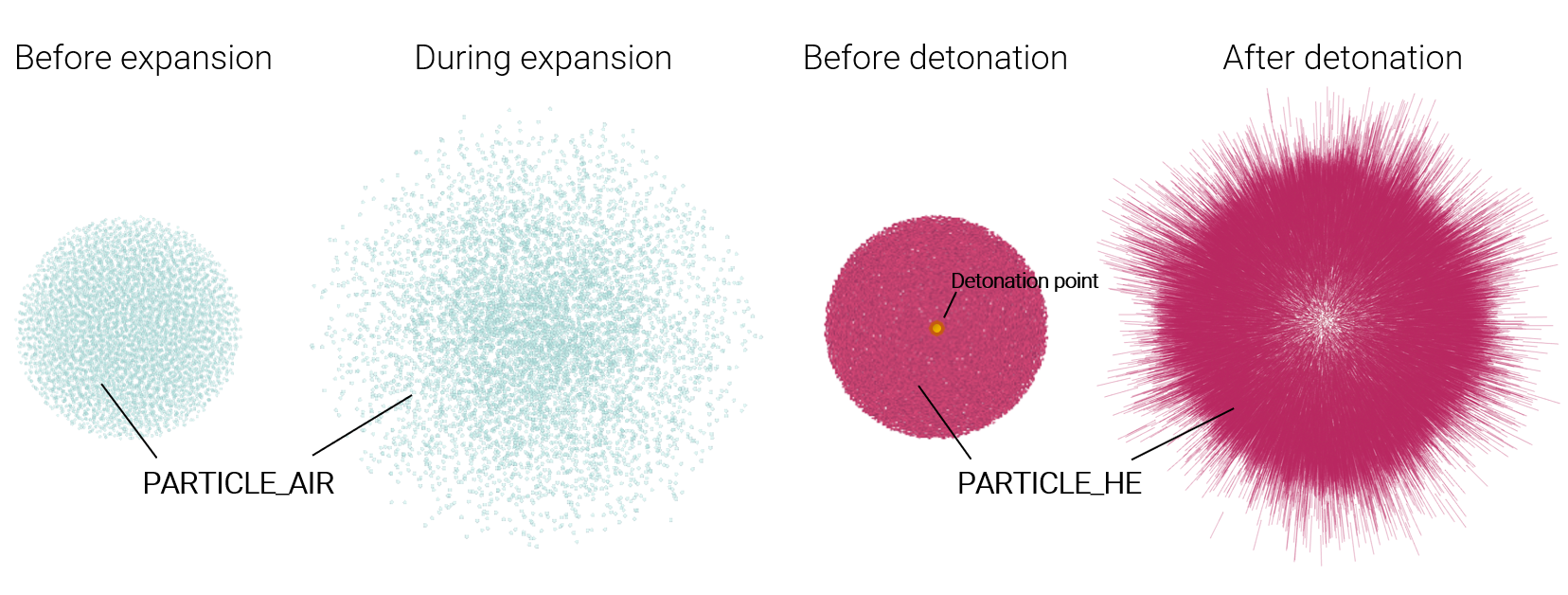
Velocity vs. time can be seen in Figure 2.
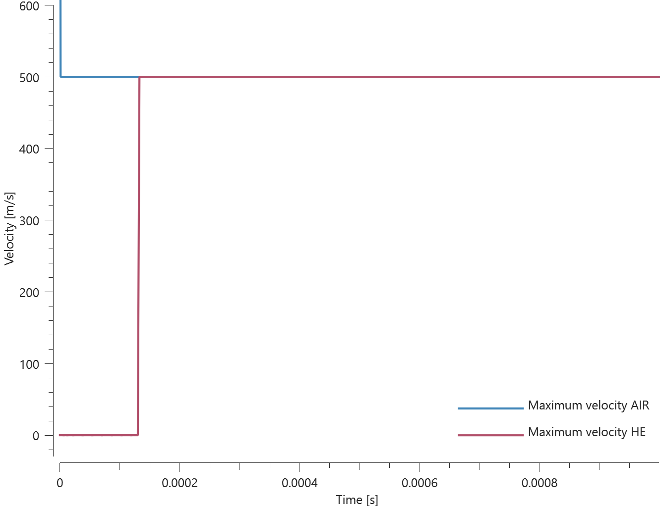
Maximum velocity is checked for version control.
Tests
This benchmark is associated with 1 tests.
CFD
$v_{max}^{N}$, $v_{max}^{DP1}$, $v_{max}^{DP2}$, $v_{max}^{CFD}$
Tested parameters: $v_{max}^{CFD}$.
This model tests maximum allowed CFD velocities for high explosives and air with the command *VELOCITY_CAP. A spherical CFD high explosives subdomain of TNT is detonated which generates extreme velocities. Also, a spherical CFD subdomain of air is expanding, surrounded by vacuum. An upper limit of $500 \ m/s$ is set to $v_{max}^{CFD}$ which prevents the AIR and HE reaching higher levels of velocity. See Figure 1.
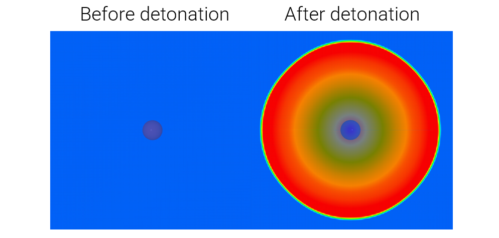
Maximum velocity in the CFD domain can be seen in Figure 2.
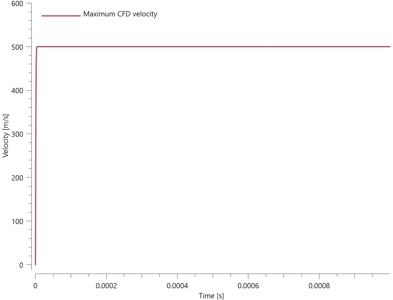
Maximum velocity is checked for version control.
Tests
This benchmark is associated with 1 tests.
Nodes
$v_{max}^{N}$, $v_{max}^{DP1}$, $v_{max}^{DP2}$, $v_{max}^{CFD}$
Tested parameters: $v_{max}^{N}$.
This model tests maximum allowed node velocities with the command *VELOCITY_CAP. A spherical object is subjected to a constant acceleration, simulating a free fall. To reach high velocity in a short amount of time, the gravitational constant is scaled. An upper limit of $500 \ m/s$ is set to the parameter $v_{max}^{N}$ which prevents all nodes reaching higher levels of velocity. See Figure 1.
Velocity of the object can be seen in Figure 2.
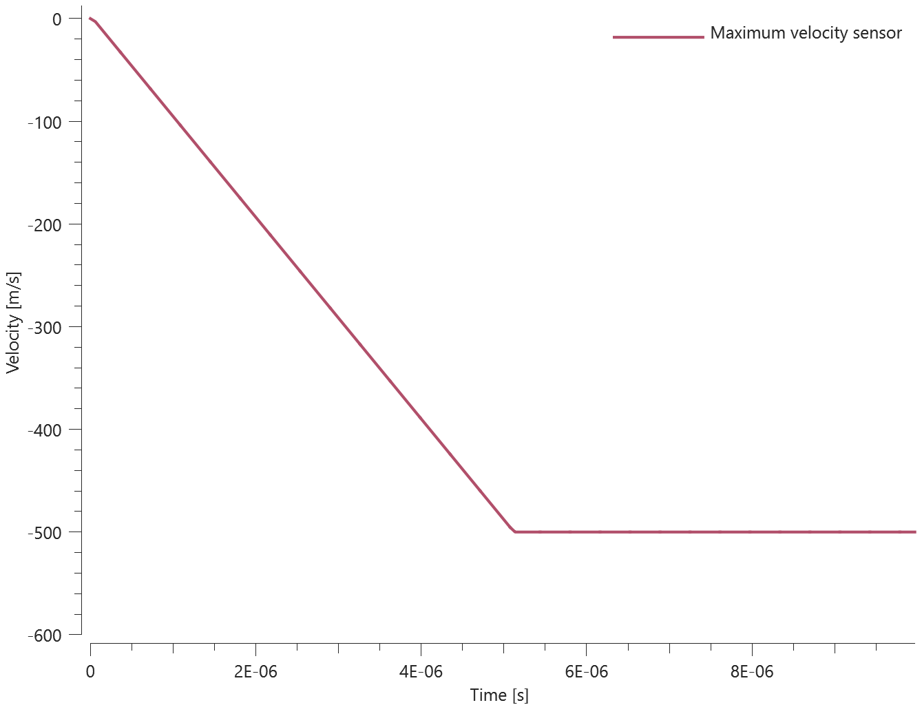
Maximum velocity is checked for version control.
Tests
This benchmark is associated with 1 tests.
SOIL and SPH
$v_{max}^{N}$, $v_{max}^{DP1}$, $v_{max}^{DP2}$, $v_{max}^{CFD}$
Tested parameters: $v_{max}^{DP1}$.
This model tests maximum allowed discrete particle and SPH velocities with the command *VELOCITY_CAP. Two spherical subdomains of SPH particles and SOIL particles are accelerated, simulating a free fall. To reach high velocity in a short amount of time, the gravitational constant is scaled. An upper limit of $500 \ m/s$ is set to $v_{max}^{DP1}$ which prevents the particles reaching higher levels of velocity. See Figure 1.
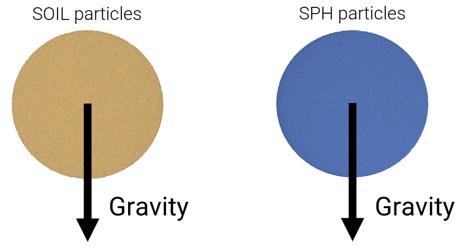
Velocity vs. time can be seen in Figure 2.
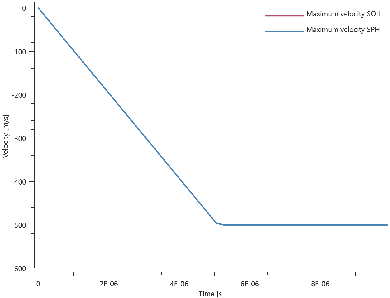
Minimum velocity is checked for version control.
Tests
This benchmark is associated with 1 tests.
*WELD
Step 1, Generate weld
nsid, stype, pid, nseg, $a$, $roff$
Tested parameters: nsid, stype, pid, nseg, $\alpha$, $roff$.
This model tests the *WELD command. It is divided into two steps, one to generate the welds and one to verify the welds. See also "*WELD - Step 2, Verify weld".
In step one the meshes of the weld seams are generated. To test the functionality of the command, two welds are created with different input parameters. The following node sets are used to define the weld paths. See Figure 1.
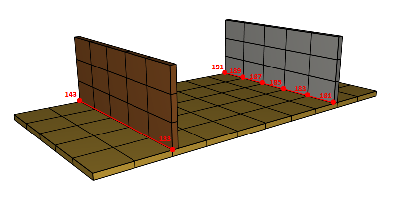
The commands below define the weld seams that are stored in weld.k under part ID's 10 and 11.
*WELD
1, 2, 10, 8, 5.0e-3
*WELD
2, 3, 11, 0, 5.0e-3, 1.0e-3
*SET_NODE
1
133, 143
*SET_NODE
2
181, 183, 185, 187, 189, 191
The number of elements along the weld path (parameter nseg) is set to 8 and 0 for the left and right weld respectively. Hence, the left weld will consist of 8 elements along its weld path and since the node set of the right weld is of 6 nodes it will consist of 5 elements in total. Different weld cross section discretization (parameter stype) is assigned. The right weld is given a root offset (parameter $roff$). The weld thickness (parameter $\alpha$) is the same for both welds. The generated weld seams can be seen in Figure 2.
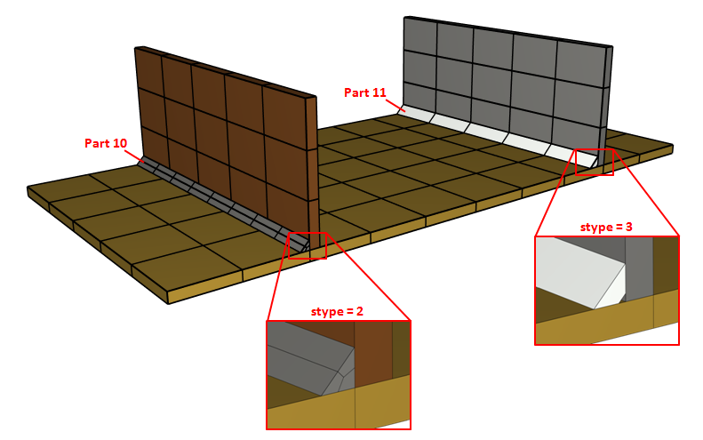
The solver terminates immediately after outputting the generated grid to the file weld.k
Tests
This benchmark is associated with 1 tests.
Step 2, Verify weld
nsid, stype, pid, nseg, $a$, $roff$
See also "*WELD - Step 1, Generate weld".
In step two the weld seams that were generated in step 1 and stored under weld.k are used. The weld geometry in weld.k can be merged with the original input using the INCLUDE command.
*INCLUDE
weld.k
*MERGE
"welds to plates"
PS, 2, PS, 1
*SET_PART
1
1, 2, 3
*SET_PART
2
10, 11
The geometry of the welds are checked for version control.
Tests
This benchmark is associated with 1 tests.