
CFD_BLAST_1D
CFD
Beta command
This command is in the beta stage and the format may change over time.
"Optional title"
coid, Stype, sid_gas, sid_exp
m_exp, R_exp, R_max, R_term, n_cells, n_dump
t_det, R_det, r_thres, i_write, dt_cfl
Parameter definition
Description
CFD_BLAST_1D is a one-dimensional CFD solver used to define the computational setup of spherically symmetric compressible flow. It applies the Harten-Lax-van Leer (HLL) Riemann solver on a uniform grid to calculate the intercell fluxes of the conserved quantities $\rho$, $\rho u$, and $E$. The HLL scheme ensures the preservation of strong and sharp shocks, which makes the solver suitable for the calculation of shock wave propagation caused by the detonation of spherical and hemispherical formed explosives. Each computational cell in the grid represents a spherical shell. The time advancement of the solver is performed explicitly. (The timestep is constrained by the Courant-Friedrichs-Lewy (CFL) condition specified in the TIME command). At the end of the simulation CFD_BLAST_1D produces a result file that can be imported into a three-dimensional CFD grid for further interactions (FSI) with embedded FE parts.
The solver supports two distinct equations of state (EOS): the Jones-Wilkins-Lee (JWL) EOS for detonation products and the ideal gas (IGE) EOS for unreacted material and surrounding air. The local EOS is selected based on a transported scalar variable, η, representing the mass fraction of burned products. This variable is advected with the flow using the same flux formulation as the conserved quantities.
In cells containing both detonation products and unreacted air, the local pressure is evaluated using a linear blending based on the burned mass fraction:
$\displaystyle{p = \eta \cdot p_{\scriptsize{\mathrm{JWL}}} + (1 - \eta) \cdot p_{\scriptsize{\mathrm{IGE}}}}$
Here, \(p_{\scriptsize{\mathrm{JWL}}}\) and \(p_{\scriptsize{\mathrm{IGE}}}\) are obtained from the respective EOS models using the local density and specific internal energy.
The specific heat at constant volume, $C_{v}$, is treated as material-dependent and constant within each phase. In mixed cells, the effective heat capacity is computed as a mass-weighted average:
$\displaystyle{C_v = \eta\cdot C_{v,p} + (1 - \eta)\cdot C_{v,g}}$
$C_{v, g}$ is the specific heat for the unreacted gas, whereas $C_{v, p}$ is the specific heat for the detonation products. Unless specified differentley in command CFD_HE, $C_{v,p}$ is set equal to $C_{v,g}$.
Temperature is obtained directly from the specific internal energy $e$ as:
$\displaystyle{T = \frac{e}{C_v}}$
The detonation of the explosive is initiated at the prescribed time and radius. After initiation, the rest of the cells containing explosive will detonate based on their distance from the initiation point and the detonation velocity of the explosive (programmed-burn). Internal energy corresponding to the specific energy of the explosive will be released into the cells through a source term during the combustion. No after-burn has been implemented so far.
Boundary conditions are imposed on the Riemann solver through ghost cells. Reflective boundary at radius 0 and open boundary at radius R_max.
Accompanying commands are CFD_GAS, CFD_HE, TIME, and OUTPUT_SENSOR. These commands are used to specify the termination time, the location of sensors and to fill the CFD domain with gases and high explosives.
Example
Air blast loaded rigid plate
The following example is of a 1 kg spherical TNT charge detonated 1.0 m above a rigid plate. The computational domain is 4 x 4 x 4 m and therefore too big to be modelled with the grid resolution needed to capture the initial shock wave formation and its propagation towards the plate. A possible solution is to model the process in two steps:
Step 1 - run the 1D solver CFD_BLAST_1D
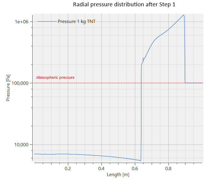
This first step utilize that everything is spherical symmetric until the shock wave hits the target plate. It can therefore be modelled i one dimension with the required grid resolution, as the numerical calculations becomes much less computationally intensive in one dimension. At termination of the simulation a text file cfd_blast_1d_coid101_mapping.k is created. This file contains information about the conserved variables at the final state of the simulation. That is density, energy, velocity, and mass fraction of combustion products in all the cells of the CFD grid.
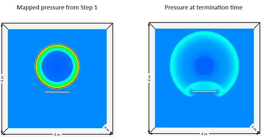
Step 2 - Map the 1D simulation results into a 3D domain. The 3D domain is filled with air by setting air=1 in CFD_DOMAIN.
The results from Step 1 are imported and mapped to a coarser three-dimensional grid to calculate the shock wave interaction with the rigid plate. The solver identifies the radial symmetry conditions from Step 1 and automatically mirrors the results to full 3D.
Sensitivity studies
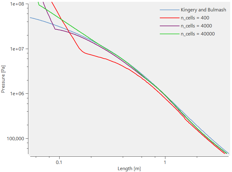
Sometimes it is convenient to perform sensitivity studies for different variables in CFD simulations to ensure a reliable numerical setup. The following example uses a 1 kg spherical TNT charge detonated in free air to investigate the grid resolution dependency of the predicted peak pressure downstream the ignition point. The results for the various grid cell sizes are compared to the overpressure reported by Kingery and Bulmash. R_max is 4.0 m.
A short tip at the end!
The i_write variable creates a binary file cfd_blast_1d_coidxxx_2D.bout which can be plotted in the PLOT section of the GUI. This makes it possible to view the transient development of the velocity, density, pressure and temperature field in the domain. That can be very useful in a number of ways.