Command manual

Elastic and viscous stresses

The total stress, $\boldsymbol{\sigma}$, is the sum of an elastic component $\boldsymbol{\sigma^e}$ and a viscous component $\boldsymbol{\sigma^v}$.

$\boldsymbol{\sigma} = \boldsymbol{\sigma^e} + \boldsymbol{\sigma^v}$

Elastic component:

$\boldsymbol{\sigma^e} = 2\cdot G\cdot \boldsymbol{\varepsilon_{dev}^e} + K\cdot \boldsymbol{\varepsilon_{vol}^e}\cdot \mathbf{I}$

$G$ is the shear modulus, $\boldsymbol{\varepsilon_{dev}^e}$ is the elastic deviatoric strain, $K$ is the bulk modulus (defined below) and $\boldsymbol{\varepsilon_{vol}^e}$ is the elastic volumetric strain.

Viscous component:

$\boldsymbol{\sigma^v} = c\cdot \boldsymbol{\dot\varepsilon}$

$c$ is an input parameter and $\boldsymbol{\dot\varepsilon}$ is the total strain rate.

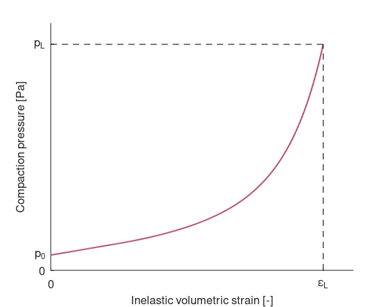
Inelastic compaction

Compaction is described by a user-defined curve of compaction pressure vs. inelastic volumetric strain. Parameters $p_0$, $p_L$ and $\varepsilon_L$ are extracted from the curve by the solver. An illustration of a compaction curve and the parameters extracted from it is presented below. The compaction pressure, $p_c\left(\varepsilon_{vol}^p\right)$, is increased gradually from $p_c\left(0\right) = p_0$ to $p_c\left(\varepsilon_L\right) = p_L$ during inelastic compaction, which occurs in region 3 (defined below).

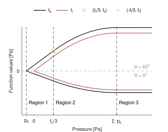
Functions $f_u$ and $f_r$

Function $f_u$ is divided into three regions, where the pressure, $p$, determines the active region.

Region 1 is active for $p \leq f_c/3$:

$f_u = max\left(0, \eta\cdot (p - p_s)\right)$

The value of $f_u$ at the transition between region 1 and 2 is denoted $f_u^{12}$.

Region 2 is active for $f_c/3 \lt p \leq \xi \cdot p_c$:

$f_u = f_u^{12} + \lambda\cdot \eta\cdot \left(\xi\cdot p_c - f_c/3 \right)\cdot \left(1 - \left(1 - \alpha\right)^{1/\lambda} \right)$

The value of $f_u$ at the transition between region 2 and 3 is denoted $f_u^{23}$.

Region 3 is active for $p \gt \xi \cdot p_c$:

$f_u = f_u^{23}$

Parameters $\eta$, $p_s$ and $\alpha$ are defined as:

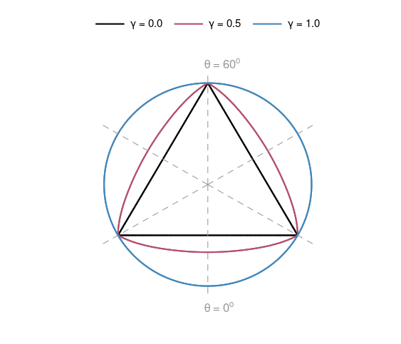
$\eta = \frac{g\left(\theta\right)\cdot f_c}{f_c/3-p_s}$

$p_s = \frac{\left(1+1/(2-\gamma)\right)\cdot f_t\cdot f_c}{3\cdot\left(f_t - f_c/(2-\gamma)\right)}$

$\alpha = \frac{p-f_c/3}{\xi\cdot p_c - f_c/3}$

Parameters $f_c$, $f_t$, $\xi$, $\lambda$ and $\gamma$ are input parameters and $g\left(\theta\right)$ is a function of Lode angle.

Function $f_r$ is defined as $f_u$ with an offset along the ordinate, leading to $f_r\left(p = 0\right) = 0$:

$f_r = max\left(0, f_u + \eta\cdot p_s\right)$

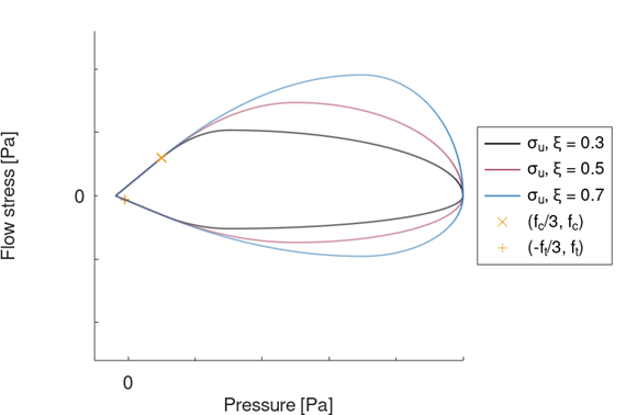
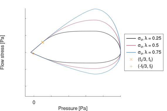
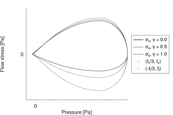
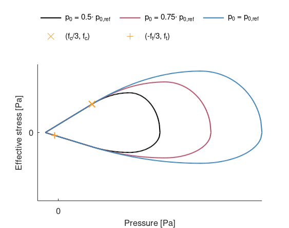
Ultimate surface

The ultimate surface, $\sigma_u$, is defined as function $f_u$ but with a cap in region 3:

$\displaystyle{\sigma_u = \left\{ \begin{array}{ccc} f_u & : & \mbox{Regions 1 and 2} \\ f_u^{23}\cdot \sqrt{1-min\left(1,\left(\frac{p-\xi\cdot p_c}{p_c\cdot (1-\xi)}\right)^2\right)} & : & \mbox{Region 3} \end{array} \right. }$

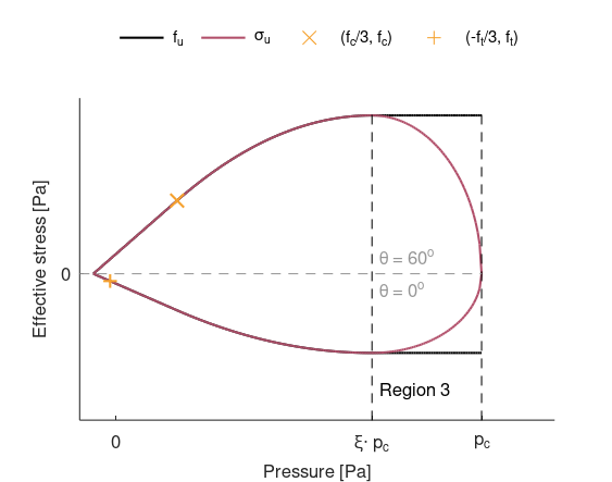
Parameters $f_c$, $f_t$, $\xi$, $\lambda$, $\gamma$ and $p_0$ control the shape of the ultimate surface.

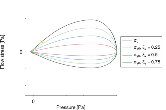
Initial yield surface

The initial yield surface, $\sigma_{y0}$, is defined based on the ultimate surface and input parameter $\xi_y$:

$\sigma_{y0} = \xi_y\cdot \sigma_u$

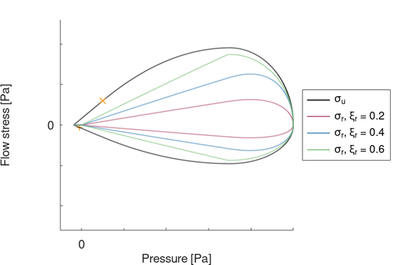
Residual surface

The residual surface, $\sigma_r$, is defined based on the ultimate surface and input parameter $\xi_r$:

$\displaystyle{\sigma_r = \left\{ \begin{array}{ccc} \beta\cdot f_r & : & \mbox{Regions 1 and 2} \\ \beta\cdot f_r^{23}\cdot \sqrt{1-min\left(1,\left(\frac{p-\xi\cdot p_c}{p_c\cdot (1-\xi)}\right)^2\right)} & : & \mbox{Region 3} \end{array} \right. }$

$\beta = min\left(1, \xi_r\cdot \eta\cdot \frac{p}{f_r}\right)$

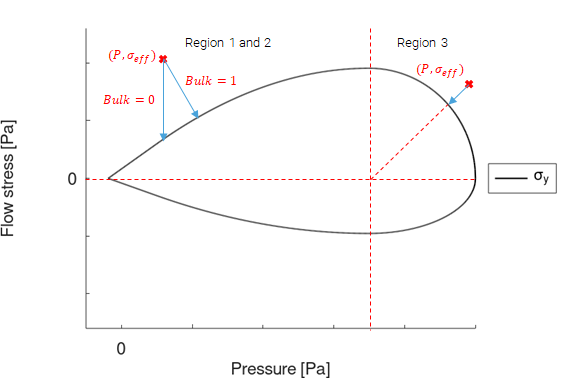
Yield criterion and plastic flow

$\begin{array}{ccc} \sigma_{eff} = \sigma_y \rightarrow \mbox{Yield} & : & \mbox{Regions 1 and 2} \\ \left(\frac{\sigma_{eff}}{\sigma_y}\right)^2 + \left(\frac{p/p_c-\xi}{1-\xi}\right)^2 \rightarrow \mbox{Yield} & : & \mbox{Region 3} \end{array}$

Parameter $bulk$ controls the return to the flow surface during plastic flow. With $bulk = 0$, the plastic flow is purely deviatoric. With $bulk = 1$, associated flow is used, meaning that the plastic flow is both deviatoric and volumetric. The volumetric strain caused by bulking can be capped with parameter $bulk_{cap}$. Bulking can only occur in regions 1 and 2. Radial return is used in region 3.

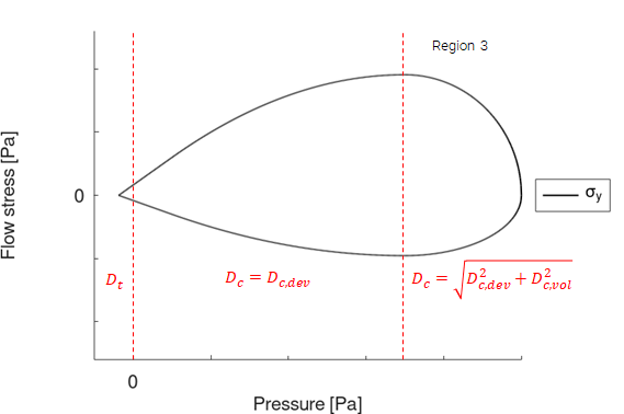
Damage

Damage is divided into tensile damage, $D_t$, and crushing damage, $D_c$. Crushing damage is divided into deviatoric crushing damage, $D_{c,dev}$, and volumetric crushing damage, $D_{c,vol}$.

Pressure and region dictate the type of damage that accumlates. Damage grows with plastic flow and is initiated once the ultimate surface is reached. Node splitting, activated with input parameter $nsplit$, is only used for tensile damage.

Tensile damage accumulates at negative pressures and does not affect the material's behavior in compression $\left(p \ge 0 \right)$.

$D_t = min\left(1,\sum{\frac{d\varepsilon_{eff}^p}{\varepsilon_{p,r}}}\right)$

Crushing damage accumulates at positive pressures and affects the material's behavior in tension $\left(p \lt 0 \right)$.

$D_c = \sqrt{D_{c,dev}^2 + D_{c,vol}^2}$

$D_{c,dev} = min\left(1,\sum{\frac{d\varepsilon_{eff}^p}{\varepsilon_{p,r}}}\right)$

$D_{c,vol} = min\left(1,\sum{\frac{d\varepsilon_{vol}^p}{\varepsilon_{L}}}\right)$

A damage factor, $D_{f}$, is defined as:

$\displaystyle{D_f = \left\{ \begin{array}{ccc} \left(1-D_c\right)^m & : & p \ge 0 \\ \left(1-D_c\right)^m\cdot \left(1-D_t\right)^m & : & p \lt 0 \end{array} \right. }$

Parameter $m$ is an input parameter.

The contour plot attribute "Damage" in the GUI displays maximum of tensile and crushing damage.

Strain rate hardening

Strain rate hardening is included with curves of strength $\left(\sigma_y^{rate}\right)$ vs. plastic strain rate $\left(\dot{\varepsilon}^p\right)$. The curve with ID $cid_{src}$ controls the hardening in compression, $p \gt f_c/3$, and the curve with ID $cid_{srt}$ controls the hardening in tension, $p \leq -f_t/3$. Linear interpolation is used for intermediate pressures.

The definition of plastic strain rate depends on region:

$\displaystyle{\dot{\varepsilon}^p = \left\{ \begin{array}{ccc} \dot{\varepsilon}_{eff}^p & : & \mbox{Regions 1 and 2} \\ \sqrt{\left(\dot{\varepsilon}_{eff}^p\right)^2 + \left(\dot{\varepsilon}_{vol}^p\right)^2} & : & \mbox{Region 3} \end{array} \right. }$

The additional strength due to strain rate hardening is added to the quasi-static strength as follows:

$\sigma_y^{dyn} = \sigma_y^{qs} + \sigma_y^{rate}\cdot D_f$

$p_c^{dyn} = p_c^{qs} + \sigma_y^{rate}\cdot D_f$

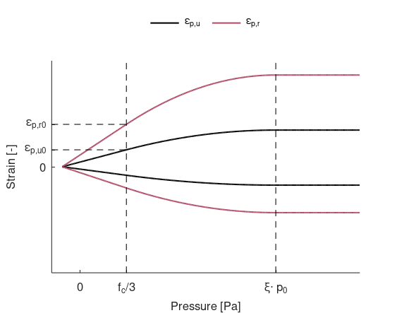
Transition: yield-ultimate surface

The transition from yield surface to ultimate surface is strain-based. The strain required in the transition is defined as:

$\varepsilon_{p,u} = \varepsilon_{p,u0}\cdot\left(1 + \psi_p\cdot \left(\frac{f_u^*+\psi_r\cdot\sigma_y^{rate}}{f_c}-1\right)\right)$

Input parameter $\varepsilon_{p,u0}$ is the strain required at $p = f_c/3$. Input parameters $\psi_p$ and $\psi_r$ controls the pressure and strain rate dependency, respectively.

The difference between function $f_u^*$ and function $f_u$ is that the former does not evolve with inelastic compaction. The two functions are therefore identical for material that has not undergone inelastic compaction, i.e., $f_u^*=f_u(p_c=p_0)$.

A lower limit on $\varepsilon_{p,u}$ can be introduced with parameter $\varepsilon_{p,u}^{min}$.

Transition: ultimate-residual surface

The transition from ultimate surface to residual surface is strain based for positive pressures. The strain required in the transition is defined as:

$\varepsilon_{p,r} = \varepsilon_{p,r0}\cdot\left(1 + \psi_p\cdot \left(\frac{f_u^*+\psi_r\cdot\sigma_y^{rate}}{f_c}-1\right)\right)$

Input parameter $\varepsilon_{p,r0}$ is the strain required at $p = f_c/3$.

At negative pressures, an energy-based transition is used if input parameter $G_{r0}$ is specified as greater than zero. A transition strain is then derived from the specified $G_{r0}$:

$\varepsilon_{p,r} = \frac{G_{r0}}{V_e^{1/3}\cdot f_c}\cdot \left(1 + \psi_p\cdot \left(\frac{f_u^*+\psi_r\cdot\sigma_y^{rate}}{f_c}-1\right)\right)$

$V_e$ is the element volume, automatically set for each element at initialization. Note that parameter $\varepsilon_{p,r0}$ must be defined even if $G_{r0} > 0$ since the energy-based transition only operates at negative pressures. The advantage of using the energy-based transition instead of the strain-based transition is that it reduces the mesh dependency.

A lower limit on $\varepsilon_{p,r}$ can be introduced with parameter $\varepsilon_{p,r}^{min}$. If the energy-based transition is used, an element reference length, $L_{ref}$, must be specified. The lower limit on $\varepsilon_{p,r}$ is then defined as $\varepsilon_{p,r}^{min}\cdot L_{ref}/V_e^{1/3}.$

Flow stress

The flow stress, $\sigma_y$, is defined as:

$\displaystyle{\sigma_y = \left\{ \begin{array}{ccc} \sigma_{y0} & : & \varepsilon_{eff}^p = 0 \mbox{ and } D_f = 1 \\ \sigma_u\cdot h & : & \varepsilon_{eff}^p \gt 0 \mbox{ and } D_f = 1 \\ \sigma_u\cdot D_f + \sigma_r\left(1-D_f\right) & : & \varepsilon_{eff}^p \gt 0 \mbox{ and } D_f \lt 1 \end{array} \right. }$

The plastic hardening, $h$, is defined as:

$h = min\left(1,\sum{\frac{d\varepsilon_{eff}^p}{\varepsilon_u}}\right), h(0) = \xi_y$

Upper and lower limits on the flow stress can be defined with input parameters $\sigma_{y,max}$ and $\sigma_{y,min}$.

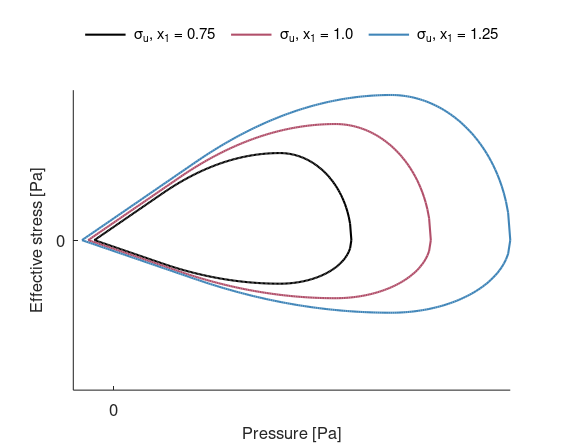
Material inhomogeneity

Deviations can be introduced with input parameter $\mu$.

$x_1 = 1 + \mu\cdot\left(2\cdot rnd - 1\right)$

$x_2 = 1 - \mu\cdot\left(2\cdot rnd - 1\right)$

$rnd$ is a random number in the interval [0,1]. Parameters $p_0$, $p_L$, $f_t$, $f_c$ are scaled with $x_1$ and parameter $\varepsilon_L$ with $x_2$. The deviations are introduced on integration point level at initialization.