MAT_FABRIC
FE
Material properties
"Optional title"
mid, $\rho$, $E$, $\nu$
$E_f$, $\varepsilon_l$, $\varepsilon_{f0}$, $\varepsilon_{f1}$, $\varepsilon_e$, $\sigma_y$, $K_n$, $n$
$\alpha_1$, $\alpha_2$, $\alpha_3$, $\alpha_4$, $\eta_1$, $\eta_2$, $\eta_3$, $\eta_4$
$\mu$, $\xi$, $c$, $\dot{\varepsilon}_0$, $W_c$
Parameter definition
Description
This is a model for fiber reinforced composites. Fibers can be defined in up to four different directions. Fiber stress, damage and failure is computed individually for each fiber direction.
A fiber stress, $\sigma_i$, is calculated as:
$\sigma_i = \left\{ \begin{array}{lcl} \displaystyle{ sf \cdot \xi \cdot \varepsilon_i } & : & \varepsilon_i \leq 0 \\ \displaystyle{ sf \cdot \left( \frac{1-\xi}{2} \cdot \frac{\varepsilon_i^2}{\varepsilon_l} + \xi \cdot \varepsilon_i \right) } & : & 0 \lt \varepsilon_i \leq \varepsilon_l \\ \displaystyle{ sf \cdot \left( \frac{\xi-1}{2} \cdot \varepsilon_l + \varepsilon_i \right) } & : & \varepsilon_i \gt \varepsilon_l \end{array} \right. $
where:
$sf = \left(1-D_i^2\right) \cdot E_f$
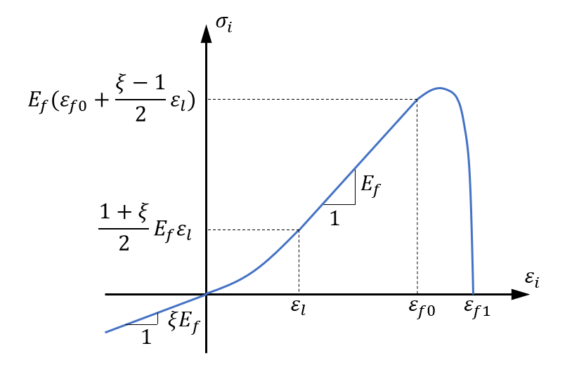
$\xi$ is the ratio between initial and full tensile stiffness for the in-plane directions. $\varepsilon_i$ is the fiber strain in the direction $i$ and $\varepsilon_i$ is the locking strain. $\varepsilon_l$ is used when modeling weaves, where initial straining of the material leads to realigning of the fibers rather than strething. $\eta_i$ is the volume fraction fibers and $D_i$ is the fiber damage level which grows irreversibly from 0 to 1:
$D_i = \left\{ \begin{array}{lcl} \displaystyle{ 0 } & : & \varepsilon_i^{max} \leq \varepsilon_{f0} \\ \displaystyle{ \frac{\varepsilon_i^{max} - \varepsilon_{f0}}{\varepsilon_{f1} - \varepsilon_{f0}} } & : & \varepsilon_{f0} \lt \varepsilon_i^{max} \leq \varepsilon_{f1} \\ \displaystyle{ 1 } & : & \varepsilon_i^{max} \gt \varepsilon_{f1} \\ \end{array} \right. $
where $\varepsilon_i^{max}$ is the largest tensile strain the fibers have experienced. $\varepsilon_{f0}$ defines when fibers begin to fail and $\varepsilon_{f1}$ defines when all fibers have failed. The failure strains can be defined to be strain rate dependent:
$\displaystyle{ \varepsilon_{f0}^{sr} = \varepsilon_{f0} \cdot \left(1 + \frac{\dot{\varepsilon}_i}{\dot{\varepsilon}_0} \right)^c }$
$\displaystyle{ \varepsilon_{f1}^{sr} = \varepsilon_{f1} \cdot \left(1 + \frac{\dot{\varepsilon}_i}{\dot{\varepsilon}_0} \right)^c }$
The pressure in the material is calculated as:
$p = \left\{ \begin{array}{lcl} \displaystyle{ -K \cdot \varepsilon_v } & : & \varepsilon_v \geq 0 \\ \displaystyle{ -K \cdot \varepsilon_v + \sum_{i = 1}^4 \eta_i \cdot K_n \cdot \vert \varepsilon_v \vert ^n } & : & \varepsilon_v \lt 0 \\ \end{array} \right. $
where $K$ is the bulk modulus of the matrix and $K_n$ and $n$ are input parameters controlling the non-linear response in compression.
The total stress in the material is defined as:
$\displaystyle{ \boldsymbol{\sigma} = 2 G \boldsymbol{\varepsilon}_{dev}^e - p \mathbf{I} + \sum_{i=1}^4 \eta_i \sigma_i \mathbf{v}_i \otimes \mathbf{v}_i + 2 \mu \dot{\boldsymbol{\varepsilon}}_{dev} }$
where $\boldsymbol{\varepsilon}_{dev}^e$ is the deviatoric elastic strain in the matrix material, $\dot{\boldsymbol{\varepsilon}}_{dev}$ is the total deviatoric strain rate and $\mathbf{v}_i$ is a fiber direction.
Matrix damage evolves with plastic flow in tension:
$\displaystyle{\dot D = \frac{\mathrm{max}(0, \sigma_1) \cdot \dot\varepsilon_{eff}^p}{W_c}}$
$\sigma_1$ is the maximum principal stress in the matrix and $\dot\varepsilon_{eff}^p$ is the effective plastic strain rate. The matrix loses its ability to carry shear loads when $D=1$.
The initial fabric orientation needs to be defined using either INITIAL_MATERIAL_DIRECTION, INITIAL_MATERIAL_DIRECTION_VECTOR or INITIAL_MATERIAL_DIRECTION_WRAP.
The effective geometric erosion strain $\varepsilon_e$ is used to remove distorted elements, but it is only active for elements where all fiber directions have failed.
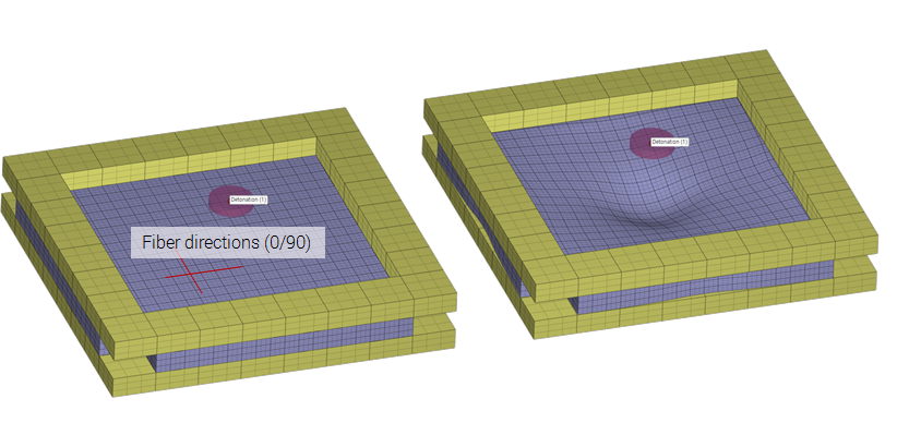
Example
Blast loaded Dyneema panel
Dyneema panel in a test rig exposed to blast loading.